Knot theory
Knot theory
Main page
2261912

Knot theory

logo
Community Hub0 subscribers
Read side by side
from Wikipedia
Examples of different knots including the trivial knot (top left) and the trefoil knot (below it)
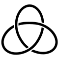
A knot diagram of the trefoil knot, the simplest non-trivial knot

In topology, knot theory is the study of mathematical knots. While inspired by knots which appear in daily life, such as those in shoelaces and rope, a mathematical knot differs in that the ends are joined so it cannot be undone, the simplest knot being a ring (or "unknot"). In mathematical language, a knot is an embedding of a circle in 3-dimensional Euclidean space, . Two mathematical knots are equivalent if one can be transformed into the other via a deformation of upon itself (known as an ambient isotopy); these transformations correspond to manipulations of a knotted string that do not involve cutting it or passing it through itself.

Knots can be described in various ways. Using different description methods, there may be more than one description of the same knot. For example, a common method of describing a knot is a planar diagram called a knot diagram, in which any knot can be drawn in many different ways. Therefore, a fundamental problem in knot theory is determining when two descriptions represent the same knot.

A complete algorithmic solution to this problem exists, which has unknown complexity.[1] In practice, knots are often distinguished using a knot invariant, a "quantity" which is the same when computed from different descriptions of a knot. Important invariants include knot polynomials, knot groups, and hyperbolic invariants.

The original motivation for the founders of knot theory was to create a table of knots and links, which are knots of several components entangled with each other. More than six billion knots and links have been tabulated since the beginnings of knot theory in the 19th century.

To gain further insight, mathematicians have generalized the knot concept in several ways. Knots can be considered in other three-dimensional spaces and objects other than circles can be used; see knot (mathematics). For example, a higher-dimensional knot is an n-dimensional sphere embedded in (n+2)-dimensional Euclidean space. Knot theory can also be extended to describe entanglement in open curves, which is used to study knots in proteins, DNA, and physical ropes.

History

[edit]
Intricate Celtic knotwork in the 1200-year-old Book of Kells

Archaeologists have discovered that knot tying dates back to prehistoric times. Besides their uses such as recording information and tying objects together, knots have interested humans for their aesthetics and spiritual symbolism. Knots appear in various forms of Chinese artwork dating from several centuries BC (see Chinese knotting). The endless knot appears in Tibetan Buddhism, while the Borromean rings have made repeated appearances in different cultures, often representing strength in unity. The Celtic monks who created the Book of Kells lavished entire pages with intricate Celtic knotwork.

The first knot tabulator, Peter Guthrie Tait

A mathematical theory of knots was first developed in 1771 by Alexandre-Théophile Vandermonde who explicitly noted the importance of topological features when discussing the properties of knots related to the geometry of position. Mathematical studies of knots began in the 19th century with Carl Friedrich Gauss, who defined the linking integral (Silver 2006). In the 1860s, Lord Kelvin's theory that atoms were knots in the aether led to Peter Guthrie Tait's creation of the first knot tables for complete classification. Tait, in 1885, published a table of knots with up to ten crossings, and what came to be known as the Tait conjectures. This record motivated the early knot theorists, but knot theory eventually became part of the emerging subject of topology.

These topologists in the early part of the 20th century—Max Dehn, J. W. Alexander, and others—studied knots from the point of view of the knot group and invariants from homology theory such as the Alexander polynomial. This would be the main approach to knot theory until a series of breakthroughs transformed the subject.

In the late 1970s, William Thurston introduced hyperbolic geometry into the study of knots with the hyperbolization theorem. Many knots were shown to be hyperbolic knots, enabling the use of geometry in defining new, powerful knot invariants. The discovery of the Jones polynomial by Vaughan Jones in 1984 (Sossinsky 2002, pp. 71–89), and subsequent contributions from Edward Witten, Maxim Kontsevich, Louis Kauffman, and others, revealed deep connections between knot theory and mathematical methods in statistical mechanics and quantum field theory. A plethora of knot invariants have been invented since then, utilizing sophisticated tools such as quantum groups and Floer homology.

In the last several decades of the 20th century, scientists became interested in studying physical knots in order to understand knotting phenomena in DNA and other polymers. Knot theory can be used to determine if a molecule is chiral (has a "handedness") or not (Simon 1986). Tangles, strings with both ends fixed in place, have been effectively used in studying the action of topoisomerase on DNA (Flapan 2000). Knot theory may be crucial in the construction of quantum computers, through the model of topological quantum computation (Collins 2006).

Knot equivalence

[edit]
On the left, the unknot, and a knot equivalent to it. It can be more difficult to determine whether complex knots, such as the one on the right, are equivalent to the unknot.

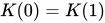
A knot is created by beginning with a one-dimensional line segment, wrapping it around itself arbitrarily, and then fusing its two free ends together to form a closed loop (Adams 2004) (Sossinsky 2002). Simply, we can say a knot is a "simple closed curve" (see Curve) — that is: a "nearly" injective and continuous function , with the only "non-injectivity" being . Topologists consider knots and other entanglements such as links and braids to be equivalent if the knot can be pushed about smoothly, without intersecting itself, to coincide with another knot.

The idea of knot equivalence is to give a precise definition of when two knots should be considered the same even when positioned quite differently in space. A formal mathematical definition is that two knots are equivalent if there is an orientation-preserving homeomorphism with .

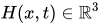
What this definition of knot equivalence means is that two knots are equivalent when there is a continuous family of homeomorphisms of space onto itself, such that the last one of them carries the first knot onto the second knot. (In detail: Two knots and are equivalent if there exists a continuous mapping such that a) for each the mapping taking to is a homeomorphism of onto itself; b) for all ; and c) . Such a function is known as an ambient isotopy.)

These two notions of knot equivalence agree exactly about which knots are equivalent: Two knots that are equivalent under the orientation-preserving homeomorphism definition are also equivalent under the ambient isotopy definition, because any orientation-preserving homeomorphisms of to itself is the final stage of an ambient isotopy starting from the identity. Conversely, two knots equivalent under the ambient isotopy definition are also equivalent under the orientation-preserving homeomorphism definition, because the (final) stage of the ambient isotopy must be an orientation-preserving homeomorphism carrying one knot to the other.

One may try to define knot equivalence based on 'isotopy' instead of the more restricted property of ambient isotopy. That is, two knots are isotopic when there exists a continuous function starting at giving the embedding, ending at giving the embedding, with all intermediate values corresponding to embeddings. However, this definition would make every knot equivalent to the unknot, as the knotted portions can be "contracted" down to a straight line. The problem is that, while continuous, this is not an injective function of the euclidean space that the knot is embedded in. Requiring that the homotopy be through homeomorphisms fixes this problem.

The basic problem of knot theory, the recognition problem, is determining the equivalence of two knots. Algorithms exist to solve this problem, with the first given by Wolfgang Haken in the late 1960s (Hass 1998). Nonetheless, these algorithms can be extremely time-consuming, and a major issue in the theory is to understand how hard this problem really is (Hass 1998). The special case of recognizing the unknot, called the unknotting problem, is of particular interest (Hoste 2005). In February 2021 Marc Lackenby announced a new unknot recognition algorithm that runs in quasi-polynomial time.[2]

Knot diagrams

[edit]
Tenfold Knottiness, plate IX, from Peter Guthrie Tait's article "On Knots", 1884

A useful way to visualise and manipulate knots is to project the knot onto a plane—think of the knot casting a shadow on the wall. A small change in the direction of projection will ensure that it is one-to-one except at the double points, called crossings, where the "shadow" of the knot crosses itself once transversely (Rolfsen 1976). At each crossing, to be able to recreate the original knot, the over-strand must be distinguished from the under-strand. This is often done by creating a break in the strand going underneath. The resulting diagram is an immersed plane curve with the additional data of which strand is over and which is under at each crossing. (These diagrams are called knot diagrams when they represent a knot and link diagrams when they represent a link.) Analogously, knotted surfaces in 4-space can be related to immersed surfaces in 3-space.

A reduced diagram is a knot diagram in which there are no reducible crossings (also nugatory or removable crossings), or in which all of the reducible crossings have been removed.[3][4] A petal projection is a type of projection in which, instead of forming double points, all strands of the knot meet at a single crossing point, connected to it by loops forming non-nested "petals".[5]

Reidemeister moves

[edit]

In 1927, working with this diagrammatic form of knots, J. W. Alexander and Garland Baird Briggs, and independently Kurt Reidemeister, demonstrated that two knot diagrams belonging to the same knot can be related by a sequence of three kinds of moves on the diagram, shown below. These operations, now called the Reidemeister moves, are:

  1. Twist and untwist in either direction.
  2. Move one strand completely over another.
  3. Move a strand completely over or under a crossing.
Reidemeister moves
Type I Type II
Type III

The proof that diagrams of equivalent knots are connected by Reidemeister moves relies on an analysis of what happens under the planar projection of the movement taking one knot to another. The movement can be arranged so that almost all of the time the projection will be a knot diagram, except at finitely many times when an "event" or "catastrophe" occurs, such as when more than two strands cross at a point or multiple strands become tangent at a point. A close inspection will show that complicated events can be eliminated, leaving only the simplest events: (1) a "kink" forming or being straightened out; (2) two strands becoming tangent at a point and passing through; and (3) three strands crossing at a point. These are precisely the Reidemeister moves (Sossinsky 2002, ch. 3) (Lickorish 1997, ch. 1).

Knot invariants

[edit]
A 3D print depicting the complement of the figure eight knot
by François Guéritaud, Saul Schleimer, and Henry Segerman

A knot invariant is a "quantity" that is the same for equivalent knots (Adams 2004) (Lickorish 1997) (Rolfsen 1976). For example, if the invariant is computed from a knot diagram, it should give the same value for two knot diagrams representing equivalent knots. An invariant may take the same value on two different knots, so by itself may be incapable of distinguishing all knots. An elementary invariant is tricolorability.

"Classical" knot invariants include the knot group, which is the fundamental group of the knot complement, and the Alexander polynomial, which can be computed from the Alexander invariant, a module constructed from the infinite cyclic cover of the knot complement (Lickorish 1997)(Rolfsen 1976). In the late 20th century, invariants such as "quantum" knot polynomials, Vassiliev invariants and hyperbolic invariants were discovered. These aforementioned invariants are only the tip of the iceberg of modern knot theory.

Knot polynomials

[edit]

A knot polynomial is a knot invariant that is a polynomial. Well-known examples include the Jones polynomial, the Alexander polynomial, and the Kauffman polynomial. A variant of the Alexander polynomial, the Alexander–Conway polynomial, is a polynomial in the variable z with integer coefficients (Lickorish 1997).

The Alexander–Conway polynomial is actually defined in terms of links, which consist of one or more knots entangled with each other. The concepts explained above for knots, e.g. diagrams and Reidemeister moves, also hold for links.

Consider an oriented link diagram, i.e. one in which every component of the link has a preferred direction indicated by an arrow. For a given crossing of the diagram, let be the oriented link diagrams resulting from changing the diagram as indicated in the figure:

The original diagram might be either or , depending on the chosen crossing's configuration. Then the Alexander–Conway polynomial, , is recursively defined according to the rules:

  • (where is any diagram of the unknot)

The second rule is what is often referred to as a skein relation. To check that these rules give an invariant of an oriented link, one should determine that the polynomial does not change under the three Reidemeister moves. Many important knot polynomials can be defined in this way.

The following is an example of a typical computation using a skein relation. It computes the Alexander–Conway polynomial of the trefoil knot. The yellow patches indicate where the relation is applied.

C() = C() + z C()

gives the unknot and the Hopf link. Applying the relation to the Hopf link where indicated,

C() = C() + z C()

gives a link deformable to one with 0 crossings (it is actually the unlink of two components) and an unknot. The unlink takes a bit of sneakiness:

C() = C() + z C()

which implies that C(unlink of two components) = 0, since the first two polynomials are of the unknot and thus equal.

Putting all this together will show:

Since the Alexander–Conway polynomial is a knot invariant, this shows that the trefoil is not equivalent to the unknot. So the trefoil really is "knotted".

Actually, there are two trefoil knots, called the right and left-handed trefoils, which are mirror images of each other (take a diagram of the trefoil given above and change each crossing to the other way to get the mirror image). These are not equivalent to each other, meaning that they are not amphichiral. This was shown by Max Dehn, before the invention of knot polynomials, using group theoretical methods (Dehn 1914). But the Alexander–Conway polynomial of each kind of trefoil will be the same, as can be seen by going through the computation above with the mirror image. The Jones polynomial can in fact distinguish between the left- and right-handed trefoil knots (Lickorish 1997).

Hyperbolic invariants

[edit]

William Thurston proved many knots are hyperbolic knots, meaning that the knot complement (i.e., the set of points of 3-space not on the knot) admits a geometric structure, in particular that of hyperbolic geometry. The hyperbolic structure depends only on the knot so any quantity computed from the hyperbolic structure is then a knot invariant (Adams 2004).

The Borromean rings are a link with the property that removing one ring unlinks the others.
SnapPea's cusp view: the Borromean rings complement from the perspective of an inhabitant living near the red component.

Geometry lets us visualize what the inside of a knot or link complement looks like by imagining light rays as traveling along the geodesics of the geometry. An example is provided by the picture of the complement of the Borromean rings. The inhabitant of this link complement is viewing the space from near the red component. The balls in the picture are views of horoball neighborhoods of the link. By thickening the link in a standard way, the horoball neighborhoods of the link components are obtained. Even though the boundary of a neighborhood is a torus, when viewed from inside the link complement, it looks like a sphere. Each link component shows up as infinitely many spheres (of one color) as there are infinitely many light rays from the observer to the link component. The fundamental parallelogram (which is indicated in the picture), tiles both vertically and horizontally and shows how to extend the pattern of spheres infinitely.

This pattern, the horoball pattern, is itself a useful invariant. Other hyperbolic invariants include the shape of the fundamental parallelogram, length of shortest geodesic, and volume. Modern knot and link tabulation efforts have utilized these invariants effectively. Fast computers and clever methods of obtaining these invariants make calculating these invariants, in practice, a simple task (Adams, Hildebrand & Weeks 1991).

Higher dimensions

[edit]

A knot in three dimensions can be untied when placed in four-dimensional space. This is done by changing crossings. Suppose one strand is behind another as seen from a chosen point. Lift it into the fourth dimension, so there is no obstacle (the front strand having no component there); then slide it forward, and drop it back, now in front. Analogies for the plane would be lifting a string up off the surface, or removing a dot from inside a circle.

In fact, in four dimensions, any non-intersecting closed loop of one-dimensional string is equivalent to an unknot. First "push" the loop into a three-dimensional subspace, which is always possible, though technical to explain.

Four-dimensional space occurs in classical knot theory, however, and an important topic is the study of slice knots and ribbon knots.

A notorious open problem, often attributed to Ralph Fox,[6][7] asks whether every slice knot is also ribbon. A knot is considered smoothly slice if it can be the boundary of a disk that is smoothly embedded in a four-dimensional ball. (The adjective "smoothly" is usually assumed, and smoothly slice knots are referred to as slice. There are other types of knots, such as rationally slice, which are not necessarily smoothly slice.) A ribbon knot is one that bounds a disk D immersed in the 3-sphere. All ribbon knots are known to be slice knots.

Knotting spheres of higher dimension

[edit]

Since a knot can be considered topologically a 1-dimensional sphere, the next generalization is to consider a two-dimensional sphere () embedded in 4-dimensional Euclidean space (). Such an embedding is knotted if there is no homeomorphism of onto itself taking the embedded 2-sphere to the standard "round" embedding of the 2-sphere. Suspended knots and spun knots are two typical families of such 2-sphere knots.

The mathematical technique called "general position" implies that for a given n-sphere in m-dimensional Euclidean space, if m is large enough (depending on n), the sphere should be unknotted. In general, piecewise-linear n-spheres form knots only in (n + 2)-dimensional space (Zeeman 1963), although this is no longer a requirement for smoothly knotted spheres. In fact, there are smoothly knotted -spheres in 6k-dimensional space; e.g., there is a smoothly knotted 3-sphere in (Haefliger 1962) (Levine 1965). Thus the codimension of a smooth knot can be arbitrarily large when not fixing the dimension of the knotted sphere; however, any smooth k-sphere embedded in with is unknotted. The notion of a knot has further generalisations in mathematics, see: Knot (mathematics), isotopy classification of embeddings.

Every knot in the n-sphere is the link of a real-algebraic set with isolated singularity in (Akbulut & King 1981).

An n-knot is a single embedded in . An n-link consists of k-copies of embedded in , where k is a natural number. Both the and the cases are well studied, and so is the case.[8][9]

Adding knots

[edit]
Adding two knots

Two knots can be added by cutting both knots and joining the pairs of ends. The operation is called the knot sum, or sometimes the connected sum or composition of two knots. This can be formally defined as follows (Adams 2004): consider a planar projection of each knot and suppose these projections are disjoint. Find a rectangle in the plane where one pair of opposite sides are arcs along each knot while the rest of the rectangle is disjoint from the knots. Form a new knot by deleting the first pair of opposite sides and adjoining the other pair of opposite sides. The resulting knot is a sum of the original knots. Depending on how this is done, two different knots (but no more) may result. This ambiguity in the sum can be eliminated regarding the knots as oriented, i.e. having a preferred direction of travel along the knot, and requiring the arcs of the knots in the sum are oriented consistently with the oriented boundary of the rectangle.

The knot sum of oriented knots is commutative and associative. A knot is prime if it is non-trivial and cannot be written as the knot sum of two non-trivial knots. A knot that can be written as such a sum is composite. There is a prime decomposition for knots, analogous to prime and composite numbers (Schubert 1949). For oriented knots, this decomposition is also unique. Higher-dimensional knots can also be added but there are some differences. While you cannot form the unknot in three dimensions by adding two non-trivial knots, you can in higher dimensions, at least when one considers smooth knots in codimension at least 3.

Knots can also be constructed using the circuit topology approach. This is done by combining basic units called soft contacts using five operations (Parallel, Series, Cross, Concerted, and Sub).[10][11] The approach is applicable to open chains as well and can also be extended to include the so-called hard contacts.

Tabulating knots

[edit]
A table of prime knots up to seven crossings. The knots are labeled with Alexander–Briggs notation

Traditionally, knots have been catalogued in terms of crossing number. Knot tables generally include only prime knots, and only one entry for a knot and its mirror image (even if they are different) (Hoste, Thistlethwaite & Weeks 1998). The number of nontrivial knots of a given crossing number increases rapidly, making tabulation computationally difficult (Hoste 2005, p. 20). Tabulation efforts have succeeded in enumerating over 6 billion knots and links (Hoste 2005, p. 28). The sequence of the number of prime knots of a given crossing number, up to crossing number 16, is 0, 0, 1, 1, 2, 3, 7, 21, 49, 165, 552, 2176, 9988, 46972, 253293, 1388705... (sequence A002863 in the OEIS). While exponential upper and lower bounds for this sequence are known, it has not been proven that this sequence is strictly increasing (Adams 2004).

The first knot tables by Tait, Little, and Kirkman used knot diagrams, although Tait also used a precursor to the Dowker notation. Different notations have been invented for knots which allow more efficient tabulation (Hoste 2005).

The early tables attempted to list all knots of at most 10 crossings, and all alternating knots of 11 crossings (Hoste, Thistlethwaite & Weeks 1998). The development of knot theory due to Alexander, Reidemeister, Seifert, and others eased the task of verification and tables of knots up to and including 9 crossings were published by Alexander–Briggs and Reidemeister in the late 1920s.

The first major verification of this work was done in the 1960s by John Horton Conway, who not only developed a new notation but also the Alexander–Conway polynomial (Conway 1970) (Doll & Hoste 1991). This verified the list of knots of at most 11 crossings and a new list of links up to 10 crossings. Conway found a number of omissions but only one duplication in the Tait–Little tables; however he missed the duplicates called the Perko pair, which would only be noticed in 1974 by Kenneth Perko (Perko 1974). This famous error would propagate when Dale Rolfsen added a knot table in his influential text, based on Conway's work. Conway's 1970 paper on knot theory also contains a typographical duplication on its non-alternating 11-crossing knots page and omits 4 examples — 2 previously listed in D. Lombardero's 1968 Princeton senior thesis and 2 more subsequently discovered by Alain Caudron. [see Perko (1982), Primality of certain knots, Topology Proceedings] Less famous is the duplicate in his 10 crossing link table: 2.-2.-20.20 is the mirror of 8*-20:-20. [See Perko (2016), Historical highlights of non-cyclic knot theory, J. Knot Theory Ramifications].

In the late 1990s Hoste, Thistlethwaite, and Weeks tabulated all the knots through 16 crossings (Hoste, Thistlethwaite & Weeks 1998). In 2003 Rankin, Flint, and Schermann, tabulated the alternating knots through 22 crossings (Hoste 2005). In 2020 Burton tabulated all prime knots with up to 19 crossings (Burton 2020).

Alexander–Briggs notation

[edit]

This is the most traditional notation, due to the 1927 paper of James W. Alexander and Garland B. Briggs and later extended by Dale Rolfsen in his knot table (see image above and List of prime knots). The notation simply organizes knots by their crossing number. One writes the crossing number with a subscript to denote its order amongst all knots with that crossing number. This order is arbitrary and so has no special significance (though in each number of crossings the twist knot comes after the torus knot). Links are written by the crossing number with a superscript to denote the number of components and a subscript to denote its order within the links with the same number of components and crossings. Thus the trefoil knot is notated 31 and the Hopf link is 22
1
. Alexander–Briggs names in the range 10162 to 10166 are ambiguous, due to the discovery of the Perko pair in Charles Newton Little's original and subsequent knot tables, and differences in approach to correcting this error in knot tables and other publications created after this point.[12]

Dowker–Thistlethwaite notation

[edit]
A knot diagram with crossings labelled for a Dowker sequence

The Dowker–Thistlethwaite notation, also called the Dowker notation or code, for a knot is a finite sequence of even integers. The numbers are generated by following the knot and marking the crossings with consecutive integers. Since each crossing is visited twice, this creates a pairing of even integers with odd integers. An appropriate sign is given to indicate over and undercrossing. For example, in this figure the knot diagram has crossings labelled with the pairs (1,6) (3,−12) (5,2) (7,8) (9,−4) and (11,−10). The Dowker–Thistlethwaite notation for this labelling is the sequence: 6, −12, 2, 8, −4, −10. A knot diagram has more than one possible Dowker notation, and there is a well-understood ambiguity when reconstructing a knot from a Dowker–Thistlethwaite notation.

Conway notation

[edit]

The Conway notation for knots and links, named after John Horton Conway, is based on the theory of tangles (Conway 1970). The advantage of this notation is that it reflects some properties of the knot or link.

The notation describes how to construct a particular link diagram of the link. Start with a basic polyhedron, a 4-valent connected planar graph with no digon regions. Such a polyhedron is denoted first by the number of vertices then a number of asterisks which determine the polyhedron's position on a list of basic polyhedra. For example, 10** denotes the second 10-vertex polyhedron on Conway's list.

Each vertex then has an algebraic tangle substituted into it (each vertex is oriented so there is no arbitrary choice in substitution). Each such tangle has a notation consisting of numbers and + or − signs.

An example is 1*2 −3 2. The 1* denotes the only 1-vertex basic polyhedron. The 2 −3 2 is a sequence describing the continued fraction associated to a rational tangle. One inserts this tangle at the vertex of the basic polyhedron 1*.

A more complicated example is 8*3.1.2 0.1.1.1.1.1 Here again 8* refers to a basic polyhedron with 8 vertices. The periods separate the notation for each tangle.

Any link admits such a description, and it is clear this is a very compact notation even for very large crossing number. There are some further shorthands usually used. The last example is usually written 8*3:2 0, where the ones are omitted and kept the number of dots excepting the dots at the end. For an algebraic knot such as in the first example, 1* is often omitted.

Conway's pioneering paper on the subject lists up to 10-vertex basic polyhedra of which he uses to tabulate links, which have become standard for those links. For a further listing of higher vertex polyhedra, there are nonstandard choices available.

Gauss code

[edit]

Gauss code, similar to the Dowker–Thistlethwaite notation, represents a knot with a sequence of integers. However, rather than every crossing being represented by two different numbers, crossings are labeled with only one number. When the crossing is an overcrossing, a positive number is listed. At an undercrossing, a negative number. For example, the trefoil knot in Gauss code can be given as: 1,−2,3,−1,2,−3

Gauss code is limited in its ability to identify knots. This problem is partially addressed with by the extended Gauss code.

See also

[edit]

References

[edit]

Further reading

[edit]
[edit]
Revisions and contributorsEdit on WikipediaRead on Wikipedia
from Grokipedia
Knot theory is a branch of mathematical topology that studies embeddings of circles (known as knots) in three-dimensional Euclidean space, focusing on their properties under continuous deformations that do not allow the curve to pass through itself.[1] These deformations, called ambient isotopies, preserve the knot's topology while allowing stretching, twisting, and shrinking, with the central problem being to determine whether two given knots are equivalent under such transformations.[2] Formally, a knot is defined as a smooth embedding of the circle $ S^1 $ into $ \mathbb{R}^3 $, or equivalently, a simple closed curve that is homeomorphic to $ S^1 $.[3] The origins of knot theory trace back to the late 19th century, when Scottish mathematician Peter Guthrie Tait began systematic tabulations of knots in connection with early atomic theories proposed by physicist William Thomson (Lord Kelvin), who hypothesized that atoms were knotted vortices in the ether.[4] Early work by Tait, Thomas Kirkman, and others focused on enumerating distinct knots, but progress stalled until the 1920s when J.W. Alexander introduced the first polynomial invariant, the Alexander polynomial, which assigns a Laurent polynomial to each knot to help distinguish them.[4] A major breakthrough occurred in 1984 with Vaughan Jones' discovery of the Jones polynomial, a new invariant that revealed unexpected connections to quantum field theory and revitalized the field.[5] Key concepts in knot theory include knot invariants, quantities such as polynomials or numbers that remain unchanged under ambient isotopy, enabling classification of knots; classical examples are the Jones, Alexander, and HOMFLY polynomials, alongside simpler invariants like the crossing number and unknotting number.[5] The theory also extends to links, which are collections of disjoint knots, and braids, whose closures yield knots, providing tools for computation via Reidemeister moves—three local transformations that generate all equivalent diagrams of a knot.[6] Modern developments incorporate quantum invariants derived from representations of quantum groups and categorification, which upgrades invariants to richer structures like Khovanov homology; a notable achievement was the 2020 proof by Lisa Piccirillo that the Conway knot is not slice, resolving a 50-year-old question using advanced invariants.[7] In 2025, mathematicians at the University of Nebraska-Lincoln disproved the conjecture that the unknotting number is additive for connected sums of knots.[8][9] Beyond pure mathematics, knot theory finds applications in biology, where it models DNA recombination and supercoiling processes, as enzymes like topoisomerases resolve knotted DNA strands without breakage.[10] In physics, knots appear in quantum field theories, string theory, and statistical mechanics, with invariants like the Jones polynomial linking to partition functions in models of three-dimensional gravity.[9] These interdisciplinary ties underscore knot theory's role in understanding complex structures in nature and technology, from protein folding to polymer entanglement.[11]

Basic Concepts

In knot theory, a knot is formally defined as a smooth embedding of the circle $ S^1 $ into three-dimensional Euclidean space $ \mathbb{R}^3 $.[12] Two such embeddings are considered the same knot if they are related by an ambient isotopy, a continuous family of embeddings that deforms one into the other while keeping the image a closed curve without self-intersections.[13] This definition captures the intuitive notion of a knotted loop of string, where the embedding ensures the curve is simple and closed, and ambient isotopy models flexible deformations in space without cutting or passing through itself.[14] A link generalizes the concept of a knot to multiple components and is defined as a smooth embedding of a disjoint union of finitely many circles into $ \mathbb{R}^3 $.[15] Each individual circle in the embedding forms a knot component, and the entire structure is studied up to ambient isotopy.[3] For instance, a two-component link consists of two disjoint closed curves that may be linked together or separate, distinguishing links from single knots while sharing the same topological framework.[16] Knots are classified as tame or wild based on their geometric regularity. A tame knot is one that is ambient isotopic to a polygonal knot, meaning it can be approximated by a finite number of straight-line segments forming a closed loop.[13] The unknot, which is the standard unknotted circle, and the trefoil knot, the simplest non-trivial knot with three crossings in its minimal diagram, are both examples of tame knots.[17] In contrast, a wild knot lacks this polygonal approximation and exhibits infinite complexity or irregularity at some point, such as a curve that spirals infinitely towards a point, making wild knots far more pathological and less studied in classical knot theory.[18] Basic properties of knots include orientability, chirality, and decomposition into prime or composite forms. Since knots are embeddings of the orientable manifold $ S^1 $, they are inherently orientable, but they are often equipped with a chosen orientation—a consistent direction along the curve, represented by arrows in diagrams—to facilitate the study of invariants and linking.[14] Chirality distinguishes knots that are not equivalent to their mirror images under orientation-preserving ambient isotopies; chiral knots exist in distinct left-handed and right-handed enantiomers, as exemplified by the trefoil knot, whose mirror image cannot be deformed into the original without reflection.[5] A knot is prime if it cannot be decomposed as the connected sum of two non-trivial knots, whereas a composite knot arises from such a sum, allowing a high-level factorization into simpler prime components, though the full operation is explored elsewhere.[3] The unknot, or trivial knot, is the embedding of $ S^1 $ into $ \mathbb{R}^3 $ that is ambient isotopic to the standard round circle lying in a plane.[12] Despite its simplicity, recognizing whether a given knot is the unknot—known as the unknot recognition problem—is computationally challenging; while decidable via algorithms like those developed by Haken in the 1960s using normal surface theory, the problem lies in NP and co-NP, with ongoing research into its exact complexity.[19]

Knot Diagrams

A knot projection is a continuous map from a knot, embedded in three-dimensional space, onto a plane, where the image consists of arcs that intersect only at double points, corresponding to locations where two parts of the knot overlap in the projection.[20] This projection captures the spatial arrangement of the knot but loses the three-dimensional depth information at these intersection points.[6] A regular projection is one in which exactly two arcs meet transversely at each double point, with no three or more arcs concurrent and no tangencies between arcs.[20] To resolve the ambiguity in a regular projection, a knot diagram augments it by specifying at each double point which arc passes over the other, typically indicated by unbroken lines for overcrossings and breaks or gaps for undercrossings.[21] Thus, a knot diagram represents an immersed circle in the plane with crossing data that encodes the knot's topology.[22] Crossings in a knot diagram are classified by convention as over or under based on the relative positioning in the original embedding.[13] Additionally, each crossing is assigned a sign: a positive crossing (+1) occurs when the overpassing arc, when rotated counterclockwise to align with the underpassing arc, follows the right-hand rule, while a negative crossing (-1) follows the left-hand rule.[23] This signing convention, illustrated in standard diagrams where the positive crossing has the over strand sloping upward to the right relative to the under strand, provides a consistent way to distinguish crossing types across different projections.[13] Knot diagrams can be further characterized as alternating or non-alternating depending on the sequence of over and under crossings encountered when traversing the diagram along the knot's orientation.[24] In an alternating diagram, crossings alternate strictly between over and under as the curve is followed; for example, the figure-eight knot (denoted 4_1) admits an alternating diagram with four crossings, where the pattern over-under-over-under repeats seamlessly. Non-alternating diagrams, by contrast, have sequences where the same type of crossing (over or under) occurs consecutively, often arising in more complex knots like the knot 8_19 (the simplest non-alternating prime knot), though many knots possess both types of diagrams.[24] To obtain a minimal or reduced representation, knot diagrams are simplified by eliminating unnecessary complexities, such as avoiding triple points in projections or ensuring no isolated loops at crossings, while preserving the knot type through careful manipulation.[25] Basic rules for diagram construction include selecting projections that minimize the number of double points and consistently applying over/under assignments based on the embedding's geometry, though further simplification typically requires equivalence-preserving transformations like Reidemeister moves, discussed later.[20]

Equivalence and Invariants

Reidemeister Moves and Ambient Isotopy

Ambient isotopy provides the fundamental topological notion of equivalence for knots in three-dimensional space. Two embeddings f,g:S1R3f, g: S^1 \to \mathbb{R}^3 of the circle into Euclidean space are ambient isotopic if there exists a continuous family of homeomorphisms ht:R3R3h_t: \mathbb{R}^3 \to \mathbb{R}^3, for t[0,1]t \in [0,1], such that h0h_0 is the identity, h1f=gh_1 \circ f = g, and each hth_t is orientation-preserving, ensuring the deformation avoids self-intersections by preserving the embedding property.[26] This deformation allows one knot to be continuously transformed into another without passing through itself, capturing the intuitive idea of "untangling" while maintaining the topological type.[27] To determine ambient isotopy combinatorially through knot diagrams, Reidemeister moves offer a set of local transformations that suffice to relate any two diagrams of the same knot. These moves, introduced by Kurt Reidemeister, consist of three types and generate all planar deformations corresponding to three-dimensional isotopies. Type I move involves adding or removing a single twist or untwist in a strand, creating or eliminating a small loop where the strand crosses itself once; this corresponds to rotating a portion of the knot around its axis. Type II move adds or removes a pair of nugatory crossings by overlapping two parallel strands, effectively introducing or eliminating a "bigon" without changing the linking structure. Type III move slides one strand over an existing crossing formed by two other strands, preserving the over-under information while rearranging the diagram locally. Each move can be performed in both directions and is reversible under ambient isotopy.[27] Reidemeister's theorem establishes that two knot diagrams represent ambient isotopic knots if and only if one can be transformed into the other via a finite sequence of these three Reidemeister moves combined with regular isotopies of the plane (continuous deformations without creating or destroying crossings). The proof involves showing that any ambient isotopy induces a sequence of such diagram changes during projection, and conversely, each move arises from a specific three-dimensional deformation: Type I from twisting, Type II from pulling strands apart or together, and Type III from sliding under or over. This equivalence reduces the continuous problem of isotopy to a discrete combinatorial one, allowing systematic manipulation of diagrams.[27] For links, which consist of multiple intertwined knots, the extension beyond single knots requires additional tools. Markov's theorem provides a characterization for link equivalence using braid representations: two braids have closures that are ambient isotopic links if and only if they are related by a sequence of braid isotopies and Markov moves, including stabilization (adding trivial strands), conjugation, and destabilization. This theorem, proved by Andrei Markov, bridges diagram equivalence to the Artin braid group, enabling a algebraic description of link isotopy while preserving the combinatorial spirit of Reidemeister moves for multi-component cases.[28] Although Reidemeister moves theoretically determine knot equivalence, the general problem of verifying whether two diagrams are related by such a sequence remains computationally challenging, with algorithms relying on normal surface theory that are decidable but impractical for knots with more than a modest number of crossings due to exponential growth in complexity. Knot invariants, such as polynomials or homology groups, serve as efficient checks for non-equivalence but cannot prove equivalence alone.[29]

Classical Invariants

Classical invariants in knot theory are fundamental tools developed in the early 20th century to distinguish knots that are not ambient isotopic, relying on combinatorial and algebraic properties of knot diagrams and their complements. These invariants, such as the knot group and the crossing number, provide initial methods to detect non-triviality and differences between knots without requiring advanced geometric structures. Later developments like the Alexander polynomial build on these by incorporating homological information, while quadratic refinements such as the Arf invariant and signature offer further discrimination, particularly for concordance classes.[30] The knot group, also known as the fundamental group of the knot complement, is a key algebraic invariant that captures the topological complexity of a knot KS3K \subset S^3. For a knot KK, the complement is the 3-manifold S3KS^3 \setminus K, and its fundamental group π1(S3K)\pi_1(S^3 \setminus K) is generated by loops around the knot strands. A concrete presentation, called the Wirtinger presentation, arises from a knot diagram with nn crossings, where each arc between under- and overpasses provides a generator xix_i for i=1,,ni = 1, \dots, n, and relations at each crossing enforce the local topology: if arc jj passes under arcs ii and kk, the relation is xj=xi1xkxix_j = x_i^{-1} x_k x_i or a conjugate depending on the crossing type. This presentation, introduced by Wirtinger in 1905, allows computation of the knot group from any diagram and is invariant under Reidemeister moves, though it may not be minimal.[30][15] The boundary torus of a tubular neighborhood of the knot carries the peripheral structure, consisting of meridian and longitude curves. A meridian is a simple closed curve on the boundary torus that bounds a disk in the tubular neighborhood (solid torus) but not in the knot complement. A longitude is a simple closed curve that bounds a disk in the knot complement but not in the tubular neighborhood. The knot group together with the peripheral structure (a choice of meridian and longitude) completely determines the isotopy class of a smooth knot in three dimensions, as proven by the Gordon–Luecke theorem.[31] The crossing number cr(K)\operatorname{cr}(K) of a knot KK is the minimal number of crossings over all possible diagrams of KK, serving as a basic measure of knot complexity. It is a non-negative integer invariant, with the unknot having cr(U)=0\operatorname{cr}(U) = 0, the trefoil knot cr(31)=3\operatorname{cr}(3_1) = 3, and the figure-eight knot cr(41)=4\operatorname{cr}(4_1) = 4. Computing cr(K)\operatorname{cr}(K) exactly is challenging, but for alternating knots, reduced alternating diagrams often achieve the minimum. This invariant, first systematically studied by Tait in the late 19th century, bounds other properties like the genus and helps in tabulation.[32] The Alexander polynomial ΔK(t)\Delta_K(t) is a Laurent polynomial invariant derived from the knot group or a Seifert surface. One definition abelianizes the knot group to obtain the infinite cyclic cover of the complement, whose first homology module over Z[t,t1]\mathbb{Z}[t, t^{-1}] is presented by the Alexander matrix, a minor of which yields ΔK(t)\Delta_K(t) up to units. Equivalently, for an oriented Seifert surface FF bounding KK with basis {1,,2g}\{ \ell_1, \dots, \ell_{2g} \} for H1(F;Z)H_1(F; \mathbb{Z}), the Seifert matrix AA has entries aij=lk(i,j+)a_{ij} = \operatorname{lk}(\ell_i, \ell_j^+), where j+\ell_j^+ is the positive push-off and lk\operatorname{lk} is the linking number; then ΔK(t)=det(t1/2At1/2AT)\Delta_K(t) = \det(t^{1/2} A - t^{-1/2} A^T), normalized to be positive at t=1t=1 and symmetric ΔK(t1)=ΔK(t)\Delta_K(t^{-1}) = \Delta_K(t). This polynomial, introduced by Alexander in 1928, detects the trefoil as non-trivial since ΔU(t)=1\Delta_U(t) = 1. The Seifert matrix formulation, due to Seifert in 1934, connects it to the topology of bounding surfaces.[33][34] The Arf invariant and knot signature provide quadratic enhancements to the Alexander polynomial, acting on the homology of the knot complement or Seifert surface. The Arf invariant Arf(K)Z/2Z\operatorname{Arf}(K) \in \mathbb{Z}/2\mathbb{Z} is defined via the mod-2 reduction of the Seifert form, measuring the quadratic refinement of the intersection form on H1(F;Z/2Z)H_1(F; \mathbb{Z}/2\mathbb{Z}); it vanishes for the unknot and equals 1 for the right-handed trefoil. The signature σ(K)\sigma(K) is the signature of the Hermitian form t1/2A+t1/2ATt^{1/2} A + t^{-1/2} A^T on H1(F;C)H_1(F; \mathbb{C}) at t=1t=-1, or more generally the Tristram-Levine signature function, providing an integer invariant related to the Seifert matrix eigenvalues. These invariants, with the Arf due to Murasugi's 1969 interpretation for knots and the signature formalized by Levine in the 1960s, distinguish amphichiral knots and bound concordance obstructions.[35][36] For the trefoil knot 313_1, the Alexander polynomial is Δ31(t)=t11+t\Delta_{3_1}(t) = t^{-1} - 1 + t, computed from its Wirtinger group presentation x,yxyx=yxy\langle x, y \mid x y x = y x y \rangle abelianized or from a Seifert matrix (1)\begin{pmatrix} -1 \end{pmatrix}. The figure-eight knot 414_1 has Δ41(t)=3tt1\Delta_{4_1}(t) = 3 - t - t^{-1}, arising from its group a,babab1=ba1ba1\langle a, b \mid a b a b^{-1} = b a^{-1} b a^{-1} \rangle or Seifert matrix (1101)\begin{pmatrix} -1 & -1 \\ 0 & 1 \end{pmatrix}; both examples illustrate how non-trivial polynomials confirm these knots are distinct from the unknot.[33][34]

Algebraic Invariants

Algebraic invariants in knot theory provide powerful tools for distinguishing knots beyond basic topological properties, often through polynomial or homological structures derived from knot presentations or diagrams. These invariants capture algebraic features of the knot complement or associated groups, enabling rigorous classification. Seminal developments include surfaces bounding the knot and polynomials satisfying recursive relations, with later advancements incorporating categorification for enhanced discriminatory power. Seifert surfaces are orientable surfaces in three-dimensional space whose boundary is a given knot, providing a key algebraic invariant through their topological properties. Introduced by Herbert Seifert in 1934, these surfaces can be constructed algorithmically from any knot diagram by resolving crossings into Seifert circles—disjoint circles obtained by smoothing overcrossings—and connecting them with twisted bands at the original crossing sites.[37] The Euler characteristic χ(S)\chi(S) of a Seifert surface SS is computed as χ(S)=VE+F\chi(S) = V - E + F, where VV, EE, and FF are the numbers of vertices, edges, and faces in a cell decomposition derived from the diagram, offering a computable invariant related to the knot's complexity. The genus g(S)g(S) of the surface, defined as g(S)=2χ(S)b2g(S) = \frac{2 - \chi(S) - b}{2} with bb the number of boundary components (typically 1 for knots), measures the minimal "handles" needed, and the knot genus is the infimum over all such surfaces.[37] The Alexander polynomial, an early algebraic invariant, arises from the fundamental group of the knot complement and can be computed using Fox calculus on group presentations. Developed by J.W. Alexander in 1928 as the first non-trivial polynomial invariant, it is the determinant of a minor of the Alexander matrix, obtained from the knot group's Wirtinger presentation.[38] Ralph Fox formalized its computation in the 1950s via free differential calculus, introducing Fox free derivatives /xi\partial/\partial x_i on the free group ring Z[F]\mathbb{Z}[F], where for a word ww in generators xjx_j, the derivative satisfies xk/xi=δik\partial x_k / \partial x_i = \delta_{ik} and the Leibniz rule (uv)/xi=u/xiv+uv/xi\partial(uv)/\partial x_i = \partial u/\partial x_i \cdot v + u \cdot \partial v/\partial x_i.[39] Applying the abelianization map to the Jacobian matrix of relations yields the Alexander matrix, whose greatest common divisor of (n1)×(n1)(n-1) \times (n-1) minors gives the polynomial Δ(t)\Delta(t), normalized to be symmetric Δ(t1)=Δ(t)\Delta(t^{-1}) = \Delta(t) and Δ(1)=1\Delta(1) = 1. This invariant refines classical linking numbers and detects amphichirality in some cases. The Jones polynomial, discovered by Vaughan Jones in 1984, marks a breakthrough in algebraic knot invariants, defined axiomatically through skein relations on oriented link diagrams. It satisfies V(L+)V(L)=(t1/2t1/2)V(L0)V(L_+) - V(L_-) = (t^{1/2} - t^{-1/2}) V(L_0), where L+L_+, LL_-, and L0L_0 are links differing only at a crossing (positive, negative, and smoothed, respectively), with normalization V()=1V(\bigcirc) = 1 for the unknot.[40] Louis Kauffman provided a combinatorial reformulation in 1987 using the Kauffman bracket D\langle D \rangle, an unoriented state-sum invariant where D=AD0+A1D\langle D \rangle = A \langle D_0 \rangle + A^{-1} \langle D_\infty \rangle at each crossing (smoothing to 0- or \infty-type), multiplied by (A3)w(D)(-A^3)^{-w(D)} for writhe w(D)w(D) and adjusted for orientation to yield the Jones polynomial via V(t)=f(A)V(t) = f(A) with A=t3/4A = -t^{-3/4}.[41] For the right-handed trefoil knot 313_1, the Jones polynomial is t+t3t4t + t^3 - t^4, distinguishing it from the unknot and figure-eight knot.[40] The HOMFLY-PT polynomial generalizes the Jones polynomial to a two-variable Laurent polynomial P(L;v,z)P(L; v, z), capturing both Alexander-Conway and Jones behaviors as specializations. Introduced collaboratively in 1985 by Freyd, Yetter, Hoste, Lickorish, Millett, and Ocneanu, it obeys the skein relation v1P(L+)vP(L)=zP(L0)v^{-1} P(L_+) - v P(L_-) = z P(L_0), with P()=1P(\bigcirc) = 1.[40] Setting v=t1v = t^{-1}, z=t1/2t1/2z = t^{1/2} - t^{-1/2} recovers the Jones polynomial, while v=1v=1, z=mz=\sqrt{m} yields the Alexander-Conway form, making it a unifying invariant for classical polynomials. Khovanov homology provides a categorification of the Jones polynomial, replacing the polynomial with a bigraded chain complex whose Euler characteristic recovers V(t)V(t). Developed by Mikhail Khovanov in 2000, it assigns to a link diagram a complex built from the 2n2^n-cube of resolutions, where nn is the number of crossings, with vertices as smoothings (0- or 1-resolution at each crossing) and edges connecting differing by one smoothing. The chain groups are direct sums of graded vector spaces from Frobenius algebras (e.g., polynomials modulo relations for the qq-graded structure), with differentials increasing the homological grading by 1 and quantum grading by 1 or 3, yielding homology groups Khi,j(L)Kh^{i,j}(L) such that (1)iqjdimKhi,j=V(q)\sum (-1)^i q^j \dim Kh^{i,j} = V(q). This homological invariant detects mutations and provides finer distinctions than the polynomial alone.

Geometric and Quantum Invariants

A significant class of knots in three-dimensional space are hyperbolic knots, which constitute the majority of all knots excluding torus knots and satellite knots.[42] For a hyperbolic knot KK, its complement S3KS^3 \setminus K admits a complete hyperbolic metric of finite volume, making it a hyperbolic 3-manifold.[43] This structure is determined up to isometry by an ideal triangulation of the complement, where the hyperbolic volume serves as a key invariant, computable via algorithms that solve for the shapes of ideal tetrahedra satisfying gluing conditions. The geometrization theorem, conjectured by William Thurston and proved by Grigory Perelman, classifies all 3-manifolds and has profound implications for knot complements.[43] Specifically, for a hyperbolic knot complement, Dehn filling along most slopes on the boundary torus yields another hyperbolic manifold, with only finitely many exceptional slopes producing non-hyperbolic geometries such as Seifert fibered spaces.[44] This finiteness result, established by Thurston, underscores the rigidity of hyperbolic structures under Dehn surgery, enabling the construction of diverse 3-manifolds from knot exteriors.[45] The Casson invariant provides another geometric measure for 3-manifolds arising from knot surgery, counting irreducible representations of the fundamental group into the special unitary group SU(2) up to conjugation.[46] For integral homology spheres obtained via Dehn surgery on a knot in the 3-sphere, the Casson invariant λ(M)\lambda(M) relates directly to the knot's surgery description, offering insights into the manifold's topology through formulas involving linking numbers and signatures.[47] This invariant detects distinctions among manifolds that share the same knot group, highlighting geometric properties beyond algebraic ones. Quantum invariants extend classical knot polynomials into the realm of topological quantum field theory, providing non-trivial distinctions for knots and 3-manifolds. The Reshetikhin-Turaev invariants, constructed from modular tensor categories associated to quantum groups, generalize the Jones polynomial to colored representations and extend it to links in arbitrary 3-manifolds via surgery presentations.[48] In particular, the colored Jones polynomials arise by assigning irreducible representations (colors) to knot strands, yielding a family of Laurent polynomials in a variable qq that detect hyperbolic volumes in the large-NN limit for SU(2) representations.[49] Geometric measures of knot complexity include the stick number and ropelength, which quantify minimal realizations in Euclidean space. The stick number s(K)s(K) of a knot KK is the smallest number of straight-line segments required to form a polygonal embedding of KK, providing a discrete bound on complexity that grows with crossing number.[50] Ropelength, defined as the minimal length of a knotted tube of unit radius without self-intersection, combines length and thickness to model physical ropes and yields upper bounds scaling linearly with stick number for many knots.[51] In a 2025 development, Mark Brittenham and Susan Hermiller disproved the long-standing conjecture that the unknotting number—a geometric complexity measure counting minimal crossing changes to unknot—is additive under connected sums, providing counterexamples where u(K1#K2)<u(K1)+u(K2)u(K_1 \# K_2) < u(K_1) + u(K_2) for specific knots with u(Ki)=3u(K_i) = 3.[52] This result, resolving Kirby's Problem 1.69(B), reveals non-additive behavior in knot complexity and prompts reevaluation of related invariants.[8]

Higher Dimensions and Generalizations

Higher-Dimensional Knots

In higher-dimensional knot theory, an n-knot is defined as the image of a smooth embedding of the n-sphere SnS^n into the (n+2)(n+2)-sphere Sn+2S^{n+2}, up to ambient isotopy.[53] This generalizes the classical case of 1-knots in S3S^3. For example, a 2-knot is a smoothly embedded 2-sphere in S4S^4, often referred to as a knotted surface, whose complement exhibits non-trivial topology despite the embedding being locally unknotted.[54] Such embeddings are studied in the smooth category, where the exterior (complement of a tubular neighborhood) provides the primary object of interest. One seminal construction for obtaining higher-dimensional knots from classical ones is Artin's spinning operation, introduced in 1925.[55] Given a classical knot KS3K \subset S^3, spinning rotates KK around an axis in S4S^4 (viewed as S3×IS^3 \times I with endpoints identified appropriately), yielding a 2-knot whose exterior fibers over the circle with fiber the classical knot complement. This method produces non-trivial examples, such as the spun trefoil, and extends to higher dimensions via generalizations like twist-spinning.[56] In dimensions where the codimension exceeds two, embeddings of spheres are unknotted. Specifically, all smooth embeddings of S1S^1 into S4S^4 (1-knots in 4D) are ambient isotopic to the standard unknot, as the high codimension allows general position arguments to resolve any intersections without obstruction.[57] Unknotting spheres, which are embedded hyperspheres bounding regions containing the knot, play a role in these proofs by enabling isotopies through handle decompositions. In contrast, codimension-two embeddings, like n-knots in Sn+2S^{n+2} for n2n \geq 2, resist simple unknotting due to the failure of the Whitney trick in low dimensions, leading to profound classification challenges that rely on algebraic topology.[58] Key invariants for higher-dimensional knots arise from the topology of their exteriors. Alexander duality implies that the homology of the knot exterior E(K)E(K) satisfies H~i(E(K))H~n+1i(K)\tilde{H}_i(E(K)) \cong \tilde{H}^{n+1-i}(K) for i0i \geq 0, providing cohomological information about the embedding.[53][59] Seifert hypersurfaces, which are connected, oriented (n+1)(n+1)-manifolds Fn+1Sn+2F^{n+1} \subset S^{n+2} with Fn+1=K\partial F^{n+1} = K, always exist by general position and duality arguments; they generalize Seifert surfaces and allow definition of signatures and other bilinear forms.[60] The Blanchfield form, a sesquilinear pairing on the torsion submodule of the Alexander module H1(E~(K);Z[t±1])H_1(\tilde{E}(K); \mathbb{Z}[t^{\pm 1}]), serves as a complete concordance invariant for odd-dimensional knots, linking the Seifert pairing to the infinite cyclic cover.[61] These tools, rooted in surgery theory, highlight the algebraic complexity of codimension-two classifications, where even simple homotopy equivalence of exteriors does not imply isotopy.[62]

Virtual and Welded Knots

Virtual knots generalize classical knots by allowing diagrams that incorporate both classical crossings—where strands intersect in the plane—and virtual crossings, represented as intersections without over/under information, such as a small circle around the crossing point. These diagrams model embeddings of circles into thickened surfaces, where virtual crossings correspond to intersections that occur outside the surface when stabilized in three-dimensional space. Classical knot diagrams form a subset of virtual knot diagrams, with no virtual crossings.[63] Two virtual knot diagrams are equivalent if one can be transformed into the other via a sequence of virtual Reidemeister moves, which extend the classical Reidemeister moves (RI, RII, RIII) to include operations involving virtual crossings: mixed virtual-classical moves (MV1, MV2, MV3) that adjust strands passing through both types of crossings, and purely virtual moves (VR2, VR3) that handle virtual crossings alone. Equivalence under these moves preserves the knot type, but three specific "forbidden moves" (F1, F2, F3)—which involve detours around virtual crossings—are not permitted, as they would alter the topological type. Any virtual knot can be unknoted by combining virtual Reidemeister moves with these forbidden moves, highlighting their role in distinguishing virtual from classical structures.[63] Welded knots extend virtual knots further by relaxing the equivalence relation to include one of the forbidden moves, specifically the overcrossing commute (OC) move, where an overstrand can pass freely under or over a virtual crossing without changing the knot type. This relaxation embeds classical knot theory into welded knot theory while allowing more equivalences, and welded knots are closed under this operation. Welded knots have applications to the study of braid groups, particularly through welded braids, which generalize classical braids by incorporating virtual crossings and the OC move, providing a framework for analyzing permutation representations and group extensions in low-dimensional topology. Key invariants for virtual knots include the virtual Jones polynomial, obtained by extending the Kauffman bracket polynomial to account for virtual crossings via a modified skein relation that treats virtual crossings as non-interacting. This polynomial distinguishes many virtual knots not separable by classical invariants. The arrow polynomial, a multivariable refinement, incorporates arrow assignments on classical crossings to track oriented structures, providing stronger discrimination; for example, it detects non-triviality in virtual knots with the same Jones polynomial.[63][64] Virtual knot theory connects to Khovanov homology through extensions that define chain complexes over arbitrary coefficients, incorporating virtual crossings via diagrammatic enhancements and preserving homological grading. This categorification yields torsion information beyond the Jones polynomial, with applications to detecting virtual unknotting.[65]

Knot Operations and Constructions

Connected Sums and Satellite Knots

The connected sum of two oriented knots K1K_1 and K2K_2 in the 3-sphere S3S^3 is constructed by selecting an unknotted arc in the diagram of each knot, removing an open tubular neighborhood of that arc from S3S^3, and gluing the resulting boundary tori together via an orientation-preserving homeomorphism that matches the meridians and longitudes appropriately (see Classical Invariants for definitions of these peripheral curves).[66] This operation yields a new knot K1#K2K_1 \# K_2 that is independent of the choice of arcs up to ambient isotopy.[67] Many classical knot invariants exhibit additivity under connected sum; for instance, the Alexander polynomial satisfies ΔK1#K2(t)=ΔK1(t)ΔK2(t)\Delta_{K_1 \# K_2}(t) = \Delta_{K_1}(t) \Delta_{K_2}(t), up to units in the Laurent polynomial ring.[68] A knot is termed prime if it cannot be expressed as the nontrivial connected sum of two knots, meaning any such decomposition involves the unknot as one factor.[69] The prime decomposition theorem asserts that every nontrivial knot in S3S^3 admits a unique decomposition as a connected sum of finitely many prime knots, unique up to reordering and choice of orientation.[70] This result, originally established by Horst Schubert, provides a fundamental factorization analogous to that of integers into primes and underpins much of classical knot classification.[70] Satellite knots generalize connected sums by incorporating more complex embeddings. Formally, a satellite knot arises from a companion knot JJ in S3S^3 and a pattern knot PP embedded in the interior of a solid torus VV, via a homeomorphism f:VN(J)f: V \to N(J) (where N(J)N(J) is a solid toroidal neighborhood of JJ) such that f(P)f(P) is the resulting knot and ff restricted to the boundary of VV is not isotopic to the core embedding of N(J)N(J).[71] Here, JJ serves as the companion, dictating the overall scale, while PP provides the intricate winding pattern.[72] Cable knots exemplify satellites, obtained when the pattern PP is a (p,q)(p,q)-torus knot in VV with gcd(p,q)=1\gcd(p,q)=1, yielding a knot that winds pp times meridionally and qq times longitudinally around JJ.[72][73] Torus knots are a distinguished family that reside on the surface of a standard unknotted torus embedded in S3S^3. The (p,q)(p,q)-torus knot, where pp and qq are coprime positive integers, traces a closed curve that wraps pp times around the torus's longitudinal direction and qq times around its meridional direction.[74] A parametric representation in R3\mathbb{R}^3 (identifying with S3S^3 via stereographic projection if needed) is given by
x=(R+rcos(qt))cos(pt),y=(R+rcos(qt))sin(pt),z=rsin(qt), \begin{align*} x &= (R + r \cos(q t)) \cos(p t), \\ y &= (R + r \cos(q t)) \sin(p t), \\ z &= r \sin(q t), \end{align*}
for t[0,2π]t \in [0, 2\pi] and R>r>0R > r > 0 controlling the torus geometry.[75] These operations influence knot symmetries, including invertibility and amphichirality. A knot is invertible if it is ambient isotopic to its inverse (with reversed orientation), and connected sums preserve invertibility when both summands do, though non-invertible knots exist and their connected sums can yield further non-invertible examples.[76] Amphichirality, the property of being isotopic to one's mirror image, can also arise under these constructions; for example, certain connected sums of satellites around amphichiral companions like the figure-eight knot produce amphichiral knots with specified properties.[77]

Special Knot Families

Alternating knots are defined by diagrams in which the over and under crossings alternate as one traverses the knot, allowing for a checkerboard coloring of the complementary regions.[78] This property simplifies the study of their invariants and equivalence under Reidemeister moves. A key result concerning alternating knots is the resolution of Tait's flyping conjecture, which states that any two reduced alternating diagrams of the same knot or link are connected by a finite sequence of flypes—specific moves that rotate portions of the diagram around a crossing. This conjecture was proved by Menasco and Thistlethwaite, establishing that flypes suffice for equivalence among reduced alternating diagrams and providing an algorithm to recognize them.[79] Fibered knots are those whose complements in the 3-sphere admit a fibration over the circle, with the fiber being an open surface (a punctured Seifert surface).[80] The monodromy of this fibration is the homeomorphism of the fiber induced by traversing the base circle once, which encodes the twisting along the knot and determines properties like the Alexander polynomial via the Seifert form.[81] The complement's Seifert fibration structure implies that the knot bounds a fiber surface, and the monodromy must be right-veering for certain fibered knots, as detected by knot Floer homology.[82] Pretzel knots are constructed by taking an even number of vertical strands, twisting them in columns according to integer parameters p1,p2,,pnp_1, p_2, \dots, p_n (with odd pip_i yielding knots), and connecting the top and bottom ends in a twisted manner to form a closed curve.[83] Most pretzel knots are hyperbolic, meaning their complements admit a complete hyperbolic metric of finite volume, with the exceptions being certain torus knots like the trefoil.[84] Montesinos knots generalize this by replacing the twisted columns with rational tangles, arranged in a cycle and closed to form the knot; they are denoted by parameters specifying each tangle's fraction.[85] Like pretzel knots, most Montesinos knots are hyperbolic, though some admit Seifert fibered surgeries, and their hyperbolicity follows from the arborescent nature of their tangle decompositions.[86] A slice knot bounds an embedded disk in the 4-ball, while a ribbon knot is a special case where the disk arises from a collection of ribbon moves—pushing parts of the knot through disjoint disks in the 4-ball without creating new intersections.[87] Ribbon knots are always slice, but the converse (the slice-ribbon conjecture) remains open.[88] The Fox-Milnor condition provides an algebraic obstruction: for a slice knot, the Alexander polynomial satisfies ΔK(t)=f(t)f(t1)\Delta_K(t) = f(t) f(t^{-1}) for some polynomial f(t)f(t) with integer coefficients.[89] In 2025, advances in computational knot theory have explored the complexity of ribbon knots through studies of untying operations and ribbonlength, a measure of the minimal length-to-width ratio for folded ribbon presentations. Researchers improved upper bounds on ribbonlength for small-crossing ribbon knots using new folding constructions, revealing that certain complex ribbon knots admit more efficient untying sequences than previously expected.[90] These findings, derived from combinatorial searches identifying over 1.6 million ribbon knots, highlight computational challenges in distinguishing ribbon from non-ribbon slice knots via untying complexity.[91]

Tabulation and Notation

Knot Tables and Catalogs

Knot tables provide systematic enumerations of distinct knot types, typically ordered by crossing number, the minimal number of crossings in any diagram of the knot. The Rolfsen table, published in 1976, catalogs all 165 prime knots with up to 10 crossings, excluding the unknot, and serves as a foundational reference for low-complexity knots.[92] This table accounts for the Perko pair, where two entries in an initial count of 166 were later recognized as equivalent under ambient isotopy.[69] Building on this, the Hoste-Thistlethwaite tables extend the enumeration to all 1,701,936 prime knots up to 16 crossings, completed in 1998 through collaborative computational efforts.[93] These tables include data on hyperbolic volumes for the majority of entries, which are hyperbolic knots, computed using normal surface theory in their complements to verify distinctness.[93] For example, the hyperbolic volume provides a geometric invariant that helps distinguish knots beyond diagrammatic equivalence. Link tables complement knot catalogs by enumerating prime links, with the Thistlethwaite link table listing all such links up to 13 crossings, though publicly available portions often focus on up to 11 crossings.[94] The Knot Atlas project, an ongoing online resource launched in the early 2000s, hosts these tables and associated data, including updates as recent as 2025 that incorporate enumerations of prime knots with 20 crossings.[95][96] Enumerations up to 20 crossings total 2,199,471,680 distinct prime knot types.[97][98] These resources use notation systems to label entries for easy reference across studies.[99] Computational challenges in building these tables arise from the exponential growth in the number of possible diagrams as crossing number increases, necessitating exhaustive generation and reduction techniques. Algorithms typically generate all reduced alternating diagrams first, then introduce non-alternating ones via twist additions, applying Reidemeister moves to normalize representations and filter equivalents.[93] Invariants such as the Jones polynomial and hyperbolic volume are employed to prune redundant candidates efficiently, ensuring computational feasibility up to higher crossings.[93][96] Tabulations maintain uniqueness by presenting each knot or link exactly once, up to ambient isotopy, with equivalence confirmed through a combination of diagrammatic normalization and invariant computations that detect all duplicates within the enumerated set.[93] This approach guarantees comprehensive coverage without repetition for the specified complexity bounds.[96]

Notation Systems

Notation systems in knot theory encode the structure of knot diagrams into sequences or symbols, enabling unique identification, systematic enumeration, and efficient computational manipulation without relying on graphical representations. These notations are crucial for constructing comprehensive knot tables and implementing algorithms in software for invariant calculations and equivalence checks. By representing crossings, orientations, and connectivity in a standardized form, they support the tabulation of millions of knots, as demonstrated in large-scale enumerations.[93] The Alexander-Briggs notation, developed by J. W. Alexander and G. B. Briggs in 1927, assigns labels to prime knots based on their minimal crossing number, denoted as the leading integer, followed by a subscript indicating the sequential order within that crossing class. For instance, the right-handed trefoil knot, with three crossings, is labeled 313_1, while the figure-eight knot is 414_1. This system orders knots by increasing crossing number and, within each class, by a canonical ordering derived from their projections, facilitating early tabulations up to nine crossings using homology invariants. Its simplicity makes it ideal for manual and initial computational catalogs, though it requires supplementary data for higher crossings. Dowker-Thistlethwaite (DT) codes, introduced by C. H. Dowker and M. B. Thistlethwaite in the 1980s, provide a permutation-based encoding of knot diagrams by indexing crossings during traversal. To construct a DT code, orient the knot and traverse it from an arbitrary starting point, assigning consecutive odd numbers (1, 3, 5, ..., 2n-1) to the undercrossings encountered and recording the even number paired with each odd index based on the second visit to that crossing (the overcrossing). The result is a sequence of even integers, with signs indicating over/under information for non-alternating knots; for example, the trefoil knot has DT code [4, 6, 2] in its standard alternating projection. For prime alternating diagrams, the DT code uniquely determines the diagram up to flype equivalence, making it highly suitable for computational enumeration and storage in databases like KnotScape.[93][100] Gauss codes, originating from C. F. Gauss's early work on linking numbers in the 19th century and formalized in modern knot theory, record the sequence of crossings encountered during an oriented traversal of the knot diagram. Each crossing is labeled with a unique integer from 1 to n, and the code lists these labels in order, prefixed by 'O' for overcrossing or 'U' for undercrossing, along with the direction (e.g., entering or leaving the crossing arc). A standard example for the trefoil knot is the sequence O1 U2 O3 U1 O2 U3, capturing the cyclic passage through all three crossings. This notation preserves the immersion structure and is foundational for deriving other codes like DT, though it may not distinguish mirror images without additional signs; its sequential nature aids in algorithmic reconstruction of diagrams for software implementations.[101] Conway notation, devised by J. H. Conway in 1967, employs a descriptive, tangle-based system where knots are built from rational tangles connected via algebraic operations like summation and multiplication. Tangles are 4-ended arcs, denoted by continued fractions (e.g., [3] for a single twist), and knots are formed by closing them; the trefoil, for example, is simply "3," representing a 3-twist tangle closed appropriately. This hierarchical approach allows compact representation of complex knots, such as 5_2 as [3 2], and excels in enumerating prime knots up to 11 crossings by systematically combining tangles, reducing redundancy in tabulation efforts. Its symbolic form supports recursive computations and tangle calculus for invariant derivations.[102] Braid words represent knots as closures of braids in the Artin braid group, where every knot is isotopic to the closure of some braid, per Alexander's theorem from 1923. A braid on m strands is encoded as a word in generators σi\sigma_i (positive crossings) and σi1\sigma_i^{-1} (negative), with the knot formed by connecting top to bottom endpoints; for the trefoil, a minimal representation is the closure of σ13\sigma_1^3 on two strands. This notation leverages the braid group's presentation for computational advantages, such as Markov moves to check equivalence, and is particularly useful in quantum invariant calculations via representations like the Jones polynomial. The minimal braid index (smallest m) provides a measure of knot complexity, aiding software tools for generating and distinguishing knots in large tables. These notations offer key advantages in compactness, enabling the storage and comparison of vast knot collections—such as the 1,701,936 knots up to 16 crossings tabulated using DT codes—and facilitating software implementations for automated enumeration and invariant computation. By converting diagrams to linear sequences or symbols, they minimize data requirements while preserving essential topological information, essential for advancing knot theory databases and algorithms.[93]

History and Applications

Historical Development

The origins of knot theory in the 19th century were deeply rooted in physics, particularly Lord Kelvin's (William Thomson's) vortex atom hypothesis proposed in 1867, which posited that atoms were distinct knotted configurations of swirling vortices in the luminiferous aether to explain chemical periodicity and stability. This idea motivated the Scottish physicist Peter Guthrie Tait to systematically enumerate and classify knots, beginning his work in the late 1860s as a means to catalog potential atomic structures; Tait published his first tables of prime knots up to seven crossings in 1876 and extended them to ten crossings by 1898, emphasizing amphichiral knots and resolving ambiguities in projections.[103] Tait's enumerations, while containing some errors later corrected, laid the groundwork for distinguishing knotted from unknotted curves and influenced early combinatorial approaches.[4] Complementing Tait's efforts, the Reverend Thomas Penyngton Kirkman independently compiled extensive lists of knot projections in the 1880s, sending Tait a catalog of 10-crossing knots in 1885 that helped refine the tables, though it included redundancies due to projection equivalences not fully understood at the time.[104] In the early 20th century, mathematicians built on Tait and Kirkman's tabulations to seek rudimentary knot invariants and properties distinguishing knot types, amid the field's initial combinatorial focus. The 1920s and 1930s marked a shift toward rigorous mathematical foundations, with James Waddell Alexander II introducing the Alexander polynomial in 1923 as the first non-trivial knot invariant derived from the fundamental group of the knot complement, providing a means to detect unknotting and linking.[105] Kurt Reidemeister developed his three moves in 1926, establishing equivalence classes for knot diagrams under ambient isotopy and enabling algebraic manipulations without physical models.[106] Emil Artin formalized the modern definition of a knot in 1928 as a continuous embedding of the circle into three-dimensional Euclidean space, shifting emphasis from physical vortices to pure topology and resolving ambiguities in earlier enumerations.[107] Following World War II, Ralph Fox advanced algebraic tools in knot theory during the 1950s and 1960s, developing Fox calculus for free groups and the free differential calculus to compute Alexander invariants more systematically, which facilitated the study of knot groups and torsion.[108] John Horton Conway revitalized the field in the 1960s and 1970s through his combinatorial notation system introduced in 1970 for describing knots via tangles and his normalization of the Alexander polynomial into the Conway polynomial in 1968, emphasizing recursive definitions and enabling efficient tabulations up to higher crossings. A pivotal breakthrough occurred in 1984 when Vaughan Jones discovered the Jones polynomial, a new Laurent polynomial invariant that unexpectedly detects chirality and distinguishes knots beyond the Alexander polynomial's capabilities, revolutionizing the field by linking knot theory to quantum mechanics and statistical physics.

Modern Advances and Applications

A pivotal modern development in knot theory arose from its intersection with quantum field theory, particularly Edward Witten's 1989 formulation interpreting the Jones polynomial through the Chern-Simons action in three-dimensional quantum Yang-Mills theory.[109] This approach not only provided a physical origin for the Jones invariant but also spawned the field of quantum topology, enabling the computation of knot polynomials via path integrals and inspiring further links between topology and quantum invariants.[109] Building on these foundations, categorification emerged in the early 2000s as a higher-level refinement of classical knot polynomials, with Heegaard Floer homology serving as a cornerstone. Introduced by Peter Ozsváth and Zoltán Szabó, this chain complex categorifies the Alexander polynomial and assigns graded homologies to knots that detect properties like fiberedness and L-space surgeries.[110] The absolute grading in Heegaard Floer homology further connects knot invariants to contact geometry and four-manifold topology, influencing ongoing research in low-dimensional topology.[110] Recent advances in 2024 and 2025 have extended knot theory into condensed matter and particle physics. In disordered three-dimensional metals, chemical-potential and magnetic-type disorders induce transitions between distinct knot types in nodal lines, revealing emergent topological phases under symmetry constraints. In particle physics, knotted solitons have been identified as meta-stable configurations in extensions of the Standard Model that incorporate the QCD axion, providing potential explanations for dark matter candidates. Topological data analysis has also yielded data-driven knot invariants, such as the multiscale Gauss link integral, which quantifies knot complexity in biological and physical datasets by integrating linking numbers across scales.[111] Interdisciplinary applications abound in biology and chemistry. In DNA replication, knots form during enzymatic processes, and topoisomerases resolve them to avoid replication stalling, with knot theory modeling the efficiency of these enzymes in vivo.[112] Protein structures occasionally exhibit deep knots that stabilize folds, impacting enzymatic activity and disease-related misfolding.[112] Chemically, the synthesis of molecular trefoil knots and higher-order topologies has progressed, exemplified by Jean-Pierre Sauvage's catenane and rotaxane work, which contributed to the 2016 Nobel Prize in Chemistry for molecular machines. In theoretical physics, knot theory underpins string theory via Chern-Simons terms and models QCD axions as knotted field configurations in soliton solutions. Prominent open problems continue to drive research. The Volume Conjecture, proposed by Rinat Kashaev, hypothesizes that the growth rate of the Jones polynomial at roots of unity asymptotically matches the hyperbolic volume of the knot complement, with partial verifications for specific families. Efficient algorithmic recognition of the unknot remains unresolved, despite decidability proofs, as current methods scale poorly for complex diagrams.[113]

References

User Avatar
No comments yet.