

MODFLOW
View on Wikipedia | This article has multiple issues. Please help improve it or discuss these issues on the talk page. (Learn how and when to remove these messages)
|


MODFLOW is the U.S. Geological Survey modular finite-difference flow model, which is a computer code that solves the groundwater flow equation. The program is used by hydrogeologists to simulate the flow of groundwater through aquifers. The source code is free public domain software,[1] written primarily in Fortran, and can compile and run on Microsoft Windows or Unix-like operating systems.

Since its original development in the early 1980s,[2] the USGS has made six major releases, and is now considered to be the de facto standard code for aquifer simulation. There are several actively developed commercial and non-commercial graphical user interfaces for MODFLOW.
MODFLOW was constructed in what was in 1980's called a modular design. This means it has many of the attributes of what came to be called object-oriented programming. For example, capabilities (called "packages") that simulate subsidence or lakes or streams, can easily be turned on and off and the execution time and storage requirements of those packages go away entirely. If a programmer wants to change something in MODFLOW, the clean organization makes it easy. Indeed, this kind of innovation is exactly what was anticipated when MODFLOW was designed.
Importantly, the modularity of MODFLOW makes it possible for different Packages to be written that are intended to address the same simulation goal in different ways. This allows differences of opinion about how system processes function to be tested. Such testing is an important part of multi-modeling, or alternative hypothesis testing. Models like MODFLOW make this kind of testing more definitive and controlled. This results because other aspects of the program remain the same. Tests become more definitive because they become less prone to being influenced unknowingly by other numerical and programming differences.
Groundwater flow equation
[edit]The governing partial differential equation for a confined aquifer used in MODFLOW is:
![{\displaystyle {\frac {\partial }{\partial x}}\left[K_{xx}{\frac {\partial h}{\partial x}}\right]+{\frac {\partial }{\partial y}}\left[K_{yy}{\frac {\partial h}{\partial y}}\right]+{\frac {\partial }{\partial z}}\left[K_{zz}{\frac {\partial h}{\partial z}}\right]+W=S_{S}{\frac {\partial h}{\partial t}}}](https://wikimedia.org/api/rest_v1/media/math/render/svg/ec0d3d32464413521a1ce2a53411d441e93a3c55)
where
- , and are the values of hydraulic conductivity along the x, y, and z coordinate axes (L/T)
- is the potentiometric head (L)
- is a volumetric flux per unit volume representing sources and/or sinks of water, where negative values are extractions, and positive values are injections (T−1)
- is the specific storage of the porous material (L−1); and
- is time (T)


Finite difference
[edit]The finite difference form of the partial differential in a discretized aquifer domain (represented using rows, columns and layers) is:
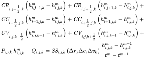
where
- is the hydraulic head at cell i,j,k at time step m
- CV, CR and CC are the hydraulic conductances, or branch conductances between node i,j,k and a neighboring node
- is the sum of coefficients of head from source and sink terms
- is the sum of constants from source and sink terms, where is flow out of the groundwater system (such as pumping) and is flow in (such as injection)
- is the specific storage
- are the dimensions of cell i,j,k, which, when multiplied, represent the volume of the cell; and
- is the time at time step m


This equation is formulated into a system of equations to be solved as:

where
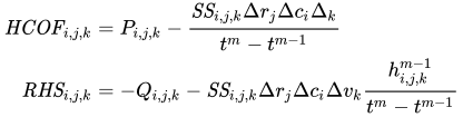
or in matrix form as:

where
- A is a matrix of the coefficients of head for all active nodes in the grid
- is a vector of head values at the end of time step m for all nodes in the grid; and
- is a vector of the constant terms, RHS, for all nodes of the grid.


Limitations
[edit]- The water must have a constant density, dynamic viscosity (and consequently temperature) throughout the modelling domain (SEAWAT is a modified version of MODFLOW which is designed for density-dependent groundwater flow and transport)
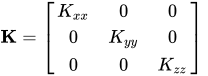
- The principal components of anisotropy of the hydraulic conductivity used in MODFLOW is displayed on the right. This tensor does not allow non-orthogonal anisotropies, as could be expected from flow in fractures. Horizontal anisotropy for an entire layer can be represented by the coefficient "TRPY" (Data Item 3 Page 153).[3]
Versions
[edit]
"Modular Model"
[edit]The USGS throughout the 1970s had developed several hundred models, written in different dialects of FORTRAN. At the time, it was common practice to rewrite a new model to fit the need of a new groundwater scenario. The concept for MODFLOW was originally designed in 1981 to provide a common modular groundwater model, which could be compiled on multiple platforms without major (or any) modification, and can read and write common formats. Different aspects of the groundwater system would be handled using the modules, similar to the idea of a "component stereo system". The original name of the code was "The USGS Modular Three-Dimensional Finite-Difference Ground-Water Flow Model", or informally as "The Modular Model". The name MODFLOW was coined several years after the initial code development, which started in 1981.[2]
The first version of MODFLOW[3] was published on December 28, 1983, and was coded entirely in FORTRAN 66. The source code for this version is listed in USGS Open File Report 83-875 referred to above.
MODFLOW-88
[edit]This version of MODFLOW[4] was rewritten in FORTRAN 77, and was originally released on July 24, 1987. The current version of MODFLOW-88 is 2.6, released on September 20, 1996.
MODPATH, was initially developed in 1989 to post-process the steady-state MODFLOW-88 data to determine three-dimensional pathlines of particles. This innovation has been indispensable for the fields of contaminant hydrogeology. It is still used as a post-processor in recent versions of MODFLOW.
A separate program, MODFLOWP, was developed in 1992 to estimate various parameters used in MODFLOW. This program was eventually built into MODFLOW-2000.
MODFLOW-96
[edit]MODFLOW-96 (version 3.0) was originally released on December 3, 1996, and is a cleaned-up and revised continuation of MODFLOW-88.[5][6] There are three final releases of MODFLOW-96:
- MODFLOW-96 (version 3.3, May 2, 2000)
- MODFLOW-96h (version 3.3h, July 10, 2000), with HYDMOD package
- MODFLOWP (version 3.2, Oct 9, 1997), MODFLOW-96 with parameter-estimation
Several graphical interfaces were first developed using the MODFLOW-96 code.
MODFLOW-2000
[edit]MODFLOW-2000 (version 1.0; version numbering was reset) was released on July 20, 2000, which merged MODFLOWP and HYDMOD codes into the main program and has integrated observation, sensitivity analysis, parameter estimation, and uncertainty evaluation capabilities.[7] Many new packages and enhancements were also included, including new solvers, stream and saturated flow packages. The internal design concepts also changed from previous versions, such that packages, processes and modules are distinct. This version was coded in a mixture of FORTRAN 77, Fortran 90, and one solver was programmed in C. MODFLOW-2000 can also be compiled for parallel computing, which can allow multiple processors to be used to increase model complexity and/or reduce simulation time. The parallelization capability is designed to support the sensitivity analysis, parameter estimation, and uncertainty analysis capabilities of MODFLOW-2000.
The final version of MODFLOW-2000 (or MF2K) is version 1.19.01, released on March 25, 2010. There are four related or branched codes based on MODFLOW-2000:
- MF2K-GWM or GWM-2000 (version 1.1.4, May 31, 2011, branched from mf2k 1.17.2), with groundwater management capability using optimization
- MF2K-FMP (version 1.00, May 19, 2006, based on mf2k 1.15.03), with Farm Process
- MF2K-GWT (version 1.9.8, October 28, 2008, based on MF2K 1.17.02), groundwater flow and solute-transport model
- SEAWAT (version 4.00.05, October 19, 2012), variable-density flow and transport processes
- VSF (version 1.01, July 5, 2006), variably saturated flow
MODFLOW-2005
[edit]MODFLOW-2005 [8] differs from MODFLOW-2000 in that the sensitivity analysis, parameter estimation, and uncertainty evaluation capabilities are removed. Thus, the support for these capabilities now falls to "clip on" codes that are supported externally to the MODFLOW support effort. In addition, the code was reorganized to support multiple models within one MODFLOW run, as needed for the LGR (Local Grid Refinement) capability.[9] MODFLOW-2005 is written primarily in Fortran 90 and C, with C being used for one solver.
The current version of MODFLOW-2005 is version 1.12.00, released on February 3, 2017. Related or branched codes include:
- MODFLOW-CFP (version 1.8.00, February 23, 2011), conduit flow process to simulate turbulent or laminar groundwater flow conditions
- MODFLOW-LGR (version 2.0, September 19, 2013), local grid refinement
- GWM-2005 (version 1.4.2, March 25, 2013), groundwater management capability using optimization
- MF2005-FMP2 (version 1.0.00, October 28, 2009), estimate dynamically integrated supply-and-demand components of irrigated agriculture as part of the simulation of surface-water and ground-water flow
- MODFLOW-NWT(version 1.1.3, August 1, 2017), Newton formulation for solving problems involving drying and rewetting nonlinearities of the unconfined groundwater-flow equation.[10]
- MODFLOW-OWHMv1[11] (version 1.00.12, October 1, 2016), The One-Water Hydrologic Flow Model (MF-OWHM1[12]), developed cooperatively between the USGS and the U.S. Bureau of Reclamation, is a fusion of multiple versions of MODFLOW-2005 (NWT, LGR, FMP, SWR, SWI) into ONE version, contains upgrades and new features and allows the simulation of head-dependent flows, flow-dependent flows, and deformation dependent flows that collectively affect conjunctive use of water resources.
- MODFLOW-USG. All version of MODFLOW listed above are constructed on what is called a structured grid. That is, the grid is composed of rectilinear blocks. The only exception is the LGR capability, which allows locally refined grids to be inserted into the structure of a "parent" grid. The local area is again composed of rectilinear blocks, but the blocks are smaller. Experimentation with a much more flexible grid structure resulted in the release of MODFLOW-USG[13] (version 1.3.00, December 1, 2015), designed to be adapted to a wide range of grid variations using unstructured grids. MODFLOW-USG has similar capabilities as MODFLOW 6, which provides grid capabilities with and intermediate level of flexibility.
- MODFLOW-USG Transport. An update of MODFLOW USG including multiple solute species transport, density dependent flow and transport, use of the Richard's equation for flow and transport in the unsaturated zone and air-water interface sorption. Some of the updates to the model have also been made to accommodate for transport of PFAS.[14][15]
MODFLOW 6
[edit]MODFLOW 6 (MF6), first released in 2017, is the sixth core version of MODFLOW to be released by the USGS.[16] This release is a rewrite of MODFLOW following an object-oriented programming paradigm in Fortran, and provides a platform that includes the capabilities from several previous MODFLOW-2005 versions, including MODFLOW-NWT, MODFLOW-USG, and MODFLOW-LGR.[17] MODFLOW 6 supports structured or unstructured grids, has full support for the Newton-Raphson formulation, and has a unique Water Mover Package that allows flows to be routed between the advanced packages, including the Streamflow Routing, Lake, Multi-Aquifer Well, and Unsaturated Zone Flow Packages. MODFLOW 6 also contains a Groundwater Transport (GWT) model that simulates transient three-dimensional solute transport on structured or unstructured grids and through the advanced flow and mover packages. An Application Programming Interface (API) is also available for MODFLOW 6, which allows the program to be coupled with other models or controlled with popular scripting languages, such as Python. While there are a few features lacking in the current release that are supported in MODFLOW-2005, most of the popular capabilities in previous MODFLOW versions are available in MODFLOW 6. The current version is 6.2.2, released July 30, 2021.[18]
MODFLOW-OWHM Version 2
[edit]The MODFLOW One-Water Hydrologic Flow Model version 2[19] (MF-OWHM) is a major rewrite of MF-OWHM1[11] released in 2020.[20] MF-OWHM is a MODFLOW-2005 based integrated hydrologic model designed for the analysis of conjunctive-use management. The term “integrated” refers to the tight coupling of groundwater flow, surface-water flow, landscape processes, aquifer compaction and subsidence, reservoir operations, and conduit (karst) flow. This fusion results in a simulation software capable of addressing water-use and sustainability problems, including conjunctive-use, water-management, water-food-security, and climate-crop-water scenarios.[21]
As a second core version of MODFLOW-2005, MF-OWHM maintains backward compatibility with existing MODFLOW-2005 versions. Existing models developed using MODFLOW-2005,[8] MODFLOW-NWT,[10] MODFLOW-SWI,[22] MODFLOW-SWR,[23] MODFLOW-LGR,[24] and MODFLOW-CFP[25] can also be simulated using MF-OWHM. The Farm Process (FMP)[26] is part of MF-OWHM but is the only component that does not maintain input backward compatibility with past releases (see the FMP_Template for new input structure). MF-OWHM also includes a Surface Water Operations Module[27] (SWO) with a Fortran-like scripting language, Slang, that can specify dynamic reservoir and stream operations. A current major application of MF-OWHM, developed by the USGS, is the California Central Valley (CVHM2).[28]
The current USGS Approved Software version is 2.3.0[29][30] released on January 15, 2024, and current preliminary-beta release of 2.3.1b-4[31] released on February 27, 2025.
Packages
[edit]The names in this table are the labels used to turn MODFLOW capabilities on and off via a key input file. Most capabilities have many alternatives or can be omitted, but the ones related to the BASIC Package are always required. Many of the capabilities introduced are supported in later versions, though the grid change enabled with MODFLOW-USG and MODFLOW 6 meant that such backward compatibility was rather selective.
| Name | Long name | Version introduced |
|---|---|---|
| Basic Package and its Components | ||
| BAS | Basic Package | original |
| OC | Output Control | original |
| DIS | Discretization | MODFLOW-2000 (1.0) |
| DISU | Unstructured Discretization | MODFLOW-USG (1.0) |
| DISV | Discretization by Vertices | MODFLOW 6 (1.00) |
| IC | Initial Conditions | MODFLOW 6 (1.00) |
| Groundwater flow packages | ||
| BCF | Block-Centered Flow Package | original |
| CLN | Connected Linear Network Process | MODFLOW-USG (1.0) |
| GNC | Ghost Node Correction Package | MODFLOW-USG (1.0) |
| HFB | Horizontal Flow Barrier Package | MODFLOW-88 |
| HUF | Hydrogeologic Unit Flow Package | MODFLOW-2000 (1.1) |
| LPF | Layer-Property Flow Package | MODFLOW-2000 (1.0) |
| NPF | Node Property Flow | MODFLOW 6 (1.00) |
| SWI2 | Seawater Intrusion Package | MODFLOW-2005 (1.11) |
| UPW | Upstream Weighting Package | MODFLOW-NWT (1.0) |
| UZF | Unsaturated-Zone Flow Package | MODFLOW-2005 (1.2) |
| Conjunctive Use and Land Use Simulation | ||
| FMP | Farm Process | MODFLOW-FMP |
| SWO | Surface Water Operations | MODFLOW-OWHM (2.0) |
| Specified Head boundary packages | ||
| CHD | Constant-Head Boundary / Time-Variant Specified-Head | MODFLOW-88 |
| FHB | Flow and Head Boundary Package | MODFLOW-96 (3.2) |
| Specified flux boundary packages | ||
| FHB | Flow and Head Boundary Package | MODFLOW-96 (3.2) |
| RCH | Recharge Package | original |
| WEL | Well Package | original |
| Head-dependent flux boundary packages | ||
| DAF | DAFLOW | MODFLOW-96 |
| DRN | Drain Package | original |
| DRT | Drain Return Package | MODFLOW-2000 (1.1) |
| ETS | Evapotranspiration Segments Package | MODFLOW-2000 (1.1) |
| EVT | Evapotranspiration Package | original |
| GHB | General-Head Boundary Package | original |
| LAK | Lake Package | MODFLOW-2000 (1.1) |
| MAW | Multi-Aquifer Well | MODFLOW 6 (1.00) |
| MNW | Multi-Node, Drawdown-Limited Well Package | MODFLOW-2000 (1.11) |
| RES | Reservoir Package | MODFLOW-88 (2.6) |
| RIP | Riparian Evapotranspiration Package | MODFLOW-OWHM (1.0) |
| RIV | River Package | original |
| SFR | Streamflow-Routing Package | MODFLOW-2000 (1.14.00) |
| STR | Stream Package | MODFLOW-88 |
| SWR | Surface-Water Routing Process | MODFLOW-NWT 1.08 |
| UZF | Unsaturated-Zone Flow Package | MODFLOW-2005 (1.2) |
| Solvers | ||
| DE4 | Direct Solver Package | MODFLOW-88 (2.5) |
| GMG | Geometric Multigrid Solver | MODFLOW-2000 (1.15.00) |
| LMG | Link-AMG Package | MODFLOW-2000 (1.4) [Note 1] |
| NWT | Newton-Raphson | MODFLOW-NWT (1.0) |
| PCG | Preconditioned Conjugate-Gradient Package | MODFLOW-88 |
| PCGN | Preconditioned Conjugate Gradient Solver with Improved Nonlinear Control | MODFLOW-2005 (1.9.0) |
| SIP | Strongly Implicit Procedure Package | original |
| SMS | Sparse Matrix Solver | MODFLOW-USG (1.0) |
| SOR | Slice Successive Over-Relaxation Package | original |
| Miscellaneous packages | ||
| GAG | Gage | MODFLOW-2000 |
| HYD | HYDMOD | MODFLOW-2000 (1.1) |
| IBS | Interbed-Storage | MODFLOW-88 |
| KDEP | Hydraulic-Conductivity Depth-Dependence Capability | MODFLOW-2000 (1.12) |
| LMT | Link-MT3DMS | MODFLOW-2000 (1.5) |
| LVDA | Model-Layer Variable-Direction Horizontal Anisotropy Capability | MODFLOW-2000 (1.12) |
| MVR | Water Mover | MODFLOW 6 (1.00) |
| STO | Storage | MODFLOW 6 (1.00) |
| SUB | Subsidence and Aquifer-System Compaction | MODFLOW-2000 (1.12) |
| SWT | Subsidence and Aquifer-System Compaction Package for Water-Table Aquifers | MODFLOW-2000 (1.18) |
| CSUB | Skeletal Storage, Compaction, and Subsidence | MODFLOW 6 (6.1.0) |
| UTL | Utility | original |
| Observation process input files | ||
| OBS | Input File For All Observations | MODFLOW-2000 |
| HOB | Head-Observation | MODFLOW-2000 |
| DROB | Drain Observation | MODFLOW-2000 |
| DTOB | Drain Return Observation | MODFLOW-2000 |
| RVOB | River Observation | MODFLOW-2000 |
| GBOB | General-Head-Boundary Observation | MODFLOW-2000 |
| CHOB | Constant-Head Flow Observation | MODFLOW-2000 |
| ADV | Advective-Transport Observation | MODFLOW-2000 (1.0) |
| STOB | Stream Observation | MODFLOW-2000 |
| Obsolete packages | ||
| GFD | General Finite-Difference | MODFLOW-88 to 96 |
| TLK | Transient Leakage | MODFLOW-88 to 96 |
- ^ Due to licensing restrictions, the USGS is no longer able to publicly distribute the Algebraic Multi-Grid
Graphical user interfaces
[edit]There are several graphical interfaces to MODFLOW, which often include the compiled MODFLOW code with modifications. These programs aid the input of data for creating MODFLOW models.
Non-commercial interfaces
[edit]Non-commercial MODFLOW versions are free, however, their licensing usually limit the use to non-profit educational or research purposes.
- ModelMuse is a grid-independent graphical user interface from the USGS for MODFLOW 6, MODPATH, SUTRA, and PHAST version 1.51. There are no license restrictions. The source code is included.
- FloPy is a Python package for creating, running, and post-processing MODFLOW-based models.
- MODFLOW-GUI – Made by the USGS: it is updated often to match the current USGS MODFLOW development. It supports MODFLOW-96, MODFLOW-2000, MODFLOW-2005, MODPATH, ZONEBUDGET, GWT, MT3DMS, SEAWAT, and GWM. Source code for MODFLOW-GUI is included. It depends on Argus ONE: a commercial interface for constructing generic models. There are no license restrictions beyond those of Argus ONE.
- PMWIN – "Processing MODFLOW" (for Windows) – powerful freeware for MODFLOW processing and visualization, provided alongside an instructional book;[32] also available in Traditional Chinese. The license for this version is limited to non-commercial use.
- mflab - mflab is a MATLAB interface to MODFLOW. The user builds and analyzes models by writing a set of MATLAB scripts. This results in flexible and efficient workflows, allowing a great deal of automation.
- iMOD - Free and open source interface developed by Deltares. iMOD contains an accelerated version of MODFLOW with fast, flexible and consistent sub-domain modeling techniques. Facilitating large, high resolution MODFLOW modeling and geo-editing of the subsurface
- FREEWAT is a free and open source, QGIS-integrated modelling platform integrating MODFLOW (MODFLOW versions integrated are MODFLOW-2005 and MODFLOW-OWHM) and the following MODFLOW-related simulation codes: MT3DMS, MT3D-USGS, SEAWAT, ZONE BUDGET, MODPATH, UCODE-2014. FREEWAT has been developed in the framework of the H2020 FREEWAT project (FREE and open source software tools for WATer resource management), financed by the EU Commission under the call WATER INNOVATION: BOOSTING ITS VALUE FOR EUROPE. The source code is released under a GNU GENERAL PUBLIC LICENSE, Version 2, June 1991, along with a complete set of User Manuals and tutorials.
Commercial programs
[edit]Commercial MODFLOW programs are typically used by governments and consultants for practical applications of MODFLOW to real-world groundwater problems. Professional versions of MODFLOW are generally priced at a minimum of around $1000 and typically range upward to US$7000. This is a list of commercial programs for MODFLOW:
- Argus ONE
- GMS – Groundwater Modeling System
- Groundwater Vistas
- Leapfrog Hydro
- Processing Modflow
- Visual MODFLOW
All current versions of these programs run only on Microsoft Windows, however previous versions of GMS (up to Version 3.1) were compiled for several Unix platforms.
Former graphical interfaces
[edit]- Graphic Groundwater – Windows-based interface
- ModelCad – A Windows-based interface, developed by Geraghty and Miller, Inc.
- ModIME Archived 2007-09-30 at the Wayback Machine – A DOS-based interface by S.S. Papadopulos & Associates, Inc.
See also
[edit]References
[edit]- ^ Water Webserver Team (March 5, 2014). "Software User Rights Notice". Water Resources of the United States. U.S. Department of the Interior, U.S. Geological Survey. Retrieved 2014-05-27.
- ^ a b McDonald M.G. & Harbaugh, A.W. (2003). "The History of MODFLOW". Ground Water. 41 (2): 280–283. Bibcode:2003GrWat..41..280M. doi:10.1111/j.1745-6584.2003.tb02591.x. PMID 12656294. S2CID 21781355.
- ^ a b c McDonald, M.G. & Harbaugh, A.W. (December 28, 1983). A modular three-dimensional finite-difference ground-water flow model. Open-File Report 83-875. U.S. Geological Survey.[permanent dead link]
- ^ McDonald, M.G. & Harbaugh, A.W. (1988). A modular three-dimensional finite-difference ground-water flow model (PDF). Techniques of Water-Resources Investigations, Book 6. U.S. Geological Survey.
- ^ Harbaugh, A.W. & McDonald, M.G. (1996a). User's documentation for MODFLOW-96, an update to the U.S. Geological Survey modular finite-difference ground-water flow model (PDF). Open-File Report 96-485. U.S. Geological Survey.
- ^ Harbaugh, A.W. & McDonald, M.G. (1996). Programmer's documentation for MODFLOW-96, an update to the U.S. Geological Survey modular finite-difference ground-water flow model (PDF). Open-File Report 96-486. U.S. Geological Survey.
- ^ Harbaugh, A.W., Banta, E.R., Hill, M.C., and McDonald, M.G. (2000). MODFLOW-2000, the U.S. Geological Survey modular ground-water model — User guide to modularization concepts and the Ground-Water Flow Process (PDF). Open-File Report 00-92. U.S. Geological Survey.
{{cite book}}: CS1 maint: multiple names: authors list (link) - ^ a b Harbaugh, Arlen W. (2005). MODFLOW-2005, The U.S. Geological Survey Modular Ground-Water Model—the Ground-Water Flow Process. Techniques and Methods 6–A16. U.S. Geological Survey.
- ^ Mehl, Steffen (2005). MODFLOW-2005, The U.S. Geological Survey Modular Ground-Water Model—Documentation of Shared Node Local Grid Refinement (LGR) and the Boundary Flow and Head (BFH) Package. Techniques and Methods 6–A12. U.S. Geological Survey.[permanent dead link]
- ^ a b Niswonger, Richard G.; Panday, Sorab; Ibaraki, Motomu (2011), "MODFLOW-NWT, A Newton Formulation for MODFLOW-2005", Techniques and Methods, Techniques and Methods 6-A37, Reston, VA: U.S. Geological Survey, doi:10.3133/tm6A37
- ^ a b Hanson, Randall T.; Boyce, Scott E.; Schmid, Wolfgang; Hughes, Joseph D.; Mehl, Steffen W.; Leake, Stanley A.; Maddock, Thomas, III; Niswonger, Richard G. (2014), "One-Water Hydrologic Flow Model (MODFLOW-OWHM)", Techniques and Methods, Techniques and Methods 6-A51, Reston, VA: U.S. Geological Survey, p. 134, doi:10.3133/tm6A51
{{citation}}: CS1 maint: multiple names: authors list (link) - ^ "Mf-Owhm | Modflow Owhm". 9 April 2020.
- ^ Panday, Sorab; Langevin, Christian D.; Niswonger, Richard G.; Ibaraki, Motomu; Hughes, Joseph D. (2013), "MODFLOW–USG Version 1: An Unstructured Grid Version of MODFLOW for Simulating Groundwater Flow and Tightly Coupled Processes Using a Control Volume Finite-Difference Formulation", USGS Report, Techniques and Methods 6-A45, Reston, VA: U.S. Geological Survey: 44, Bibcode:2013usgs.rept...44P, doi:10.3133/tm6A45
- ^ Panday, Sorab (2024); USG-Transport Version 2.4.0: Transport and Other Enhancements to MODFLOW-USG, GSI Environmental, http://www.gsi-net.com/en/software/free-software/USG-Transport.html
- ^ Hort, Hiroko M.; Stockwell, Emily B.; Newell, Charles J.; Scalia, Joseph; Panday, Sorab (2024). "Modeling and Evaluation of PFOS Retention in the Unsaturated Zone above the Water Table". Groundwater Monitoring & Remediation. 44 (3): 38–48. Bibcode:2024GMRed..44c..38H. doi:10.1111/gwmr.12662. ISSN 1069-3629.
- ^ Hughes, Joseph D.; Langevin, Christian D.; Banta, Edward R. (2017). "Documentation for the MODFLOW 6 framework". Techniques and Methods. Techniques and Methods 6-A57. p. 40. doi:10.3133/tm6A57.
- ^ Langevin, Christian D.; Hughes, Joseph D.; Banta, Edward R.; Niswonger, Richard G.; Panday, Sorab; Provost, Alden M. (2017). "Documentation for the MODFLOW 6 Groundwater Flow Model". Techniques and Methods. Techniques and Methods 6-A55. doi:10.3133/tm6A55.
- ^ "MODFLOW 6: USGS Modular Hydrologic Model".
- ^ Boyce, Scott E.; Hanson, Randall T.; Ferguson, Ian; Schmid, Wolfgang; Henson, Wesley R.; Reimann, Thomas; Mehl, Steffen W.; Earll, Marisa M. (2020). "One-Water Hydrologic Flow Model: A MODFLOW based conjunctive-use simulation software". Techniques and Methods (Report). U.S. Geological Survey. doi:10.3133/tm6a60.
- ^ Boyce, S.E., 2020, MODFLOW One-Water Hydrologic Flow Model (MF-OWHM) Conjunctive Use and Integrated Hydrologic Flow Modeling Software, version 2.0.0: U.S. Geological Survey Software Release, https://doi.org/10.5066/P9P8I8GS
- ^ "MODFLOW One-Water Hydrologic Flow Model (MF-OWHM) | U.S. Geological Survey". www.usgs.gov. 2020-04-07. Retrieved 2025-03-18.
- ^ Bakker, Mark; Schaars, Frans; Hughes, Joseph D.; Langevin, Christian D.; Dausman, Alyssa M. (2013). Documentation of the seawater intrusion (SWI2) package for MODFLOW (Report). U.S. Geological Survey.
- ^ Hughes, Joseph D.; Langevin, Christian D.; Chartier, Kevin L.; White, Jeremy T. (2012). Documentation of the Surface-Water Routing (SWR1) Process for modeling surface-water flow with the U.S. Geological Survey Modular Ground-Water Model (MODFLOW-2005) (Report). U.S. Geological Survey. pp. i–113.
- ^ Mehl, Steffen W.; Hill, Mary C. (2013). MODFLOW–LGR—Documentation of ghost node local grid refinement (LGR2) for multiple areas and the boundary flow and head (BFH2) package (Report). U.S. Geological Survey.
- ^ Shoemaker, W.B., Kuniansky, E.L., Birk, S., Bauer, S., and Swain, E.D., 2008, Documentation of a Conduit Flow Process (CFP) for MODFLOW-2005: U.S. Geological Survey Techniques and Methods, Book 6, Chapter A24, 50 p., https://pubs.usgs.gov/tm/tm6a24/
- ^ Schmid, Wolfgang, and Hanson, R.T., 2009, The Farm Process Version 2 (FMP2) for MODFLOW-2005—Modifications and Upgrades to FMP1: U.S. Geological Survey Techniques and Methods 6-A-32, 102 p., https://pubs.usgs.gov/tm/tm6a32/
- ^ Ferguson, I.M.., Llewellyn, D., Hanson, R.T., and Boyce S.E., 2016, User guide to the surface water operations process—An integrated approach to simulating large-scale surface water management in MODFLOW-based hydrologic models: Denver, Colo., Bureau of Reclamation Technical Memorandum no. 86-68210–2016-02, 96 p.
- ^ Faunt, Claudia C.; Traum, Jonathan A.; Boyce, Scott E.; Seymour, Whitney A.; Jachens, Elizabeth R.; Brandt, Justin T.; Sneed, Michelle; Bond, Sandra; Marcelli, Marina F. (2024-04-22). "Groundwater Sustainability and Land Subsidence in California's Central Valley". Water. 16 (8): 1189. Bibcode:2024Water..16.1189F. doi:10.3390/w16081189. ISSN 2073-4441.
- ^ Boyce, S.E., 2024, MODFLOW One-Water Hydrologic Flow Model (MF-OWHM) Conjunctive Use and Integrated Hydrologic Flow Modeling Software, version 2.3.0: U.S. Geological Survey Software Release, https://doi.org/10.5066/P9P8I8GS
- ^ Boyce, S.E. and Ferguson, I.M., 2024, MODFLOW One-Water Hydrologic Flow Model (MF-OWHM) Conjunctive Use and Integrated Hydrologic Flow Modeling Software with Surface Water Operations, version 2.3.0: U.S. Geological Survey Software Release, https://doi.org/10.5066/P9P8I8GS
- ^ Boyce, S.E., 2025, MODFLOW One-Water Hydrologic Flow Model (MF-OWHM) Conjunctive Use and Integrated Hydrologic Flow Modeling Software, version 2.3.1-b4: U.S. Geological Survey Software Release, https://doi.org/10.5066/P9P8I8GS
- ^ Wen-Hsing Chiang (2005). 3D-Groundwater Modeling with PMWIN (Second ed.). Springer. doi:10.1007/3-540-27592-4. ISBN 978-3-540-27590-9.
MODFLOW
View on GrokipediaOverview
Description and Purpose
MODFLOW is a modular, three-dimensional finite-difference groundwater flow model developed by the United States Geological Survey (USGS) in Fortran, designed to solve the groundwater flow equation for simulating flow in saturated porous media.[3][4] The model simulates both steady-state and transient groundwater flow conditions in confined, unconfined, and mixed aquifers, enabling analyses of hydraulic heads, flow paths, and interactions with surface water features.[3] Its primary purposes include supporting groundwater resource management for water supply planning, assessing contaminant transport and plume migration, and predicting land subsidence due to aquifer compaction.[5][6] A hallmark of MODFLOW is its modular design, which allows users to selectively activate or deactivate simulation processes—such as river-aquifer interactions via the River (RIV) package or well pumping via the Well (WEL) package—without altering the core code, facilitating customized simulations for diverse hydrogeologic settings.[3][7] The software operates on both Windows and Unix-based systems and has been freely available in the public domain since its initial release, promoting accessibility for researchers, consultants, and agencies worldwide.[3] MODFLOW has become the de facto international standard for groundwater modeling, widely adopted by hydrogeologists and integrated into geographic information systems (GIS) and other hydrologic software tools like ModelMuse and FloPy for enhanced preprocessing, simulation, and visualization.[1] As of 2025, the latest iteration, MODFLOW 6, incorporates support for unstructured grids to improve resolution in complex geometries and provides an application programming interface (API) for custom integrations, such as coupling with energy transport models.[2][8]Development History
MODFLOW was conceived in 1981 by Michael G. McDonald and Allan W. Harbaugh at the U.S. Geological Survey (USGS) as a modular three-dimensional finite-difference groundwater flow model, with the initial version completed and released in 1984 as USGS Open-File Report 83-875.[9] Written in Fortran 66, the model drew inspiration from modular designs in petroleum reservoir simulation and earlier hydrologic models to enable flexible assembly of simulation components for diverse groundwater problems.[9] This development addressed the growing need for a standardized, user-friendly tool for groundwater modeling, spurred by 1980s regulatory demands for water resource management and environmental protection, including assessments related to hazardous waste sites under programs like Superfund.[1] Key early milestones included the 1988 release of MODFLOW-88, which updated the code to Fortran 77 and provided revised documentation in USGS Techniques and Methods, book 6, chapter A1, enhancing accessibility and public adoption.[9] In 1996, MODFLOW-96 introduced a name file for improved usability and significant Fortran code refinements, broadening its application within and beyond the USGS.[9] The 2000 version, MODFLOW-2000, incorporated the "process" concept to support solute transport and parameter estimation, along with sensitivity analysis capabilities, marking a shift toward more integrated hydrologic simulations.[9] This was followed in 2005 by MODFLOW-2005, which adopted Fortran 90 with modular data management, advanced solvers, and support for nested and refined grids to handle complex spatial variability.[9] A modern paradigm shift occurred with the 2017 launch of MODFLOW 6, an object-oriented framework in Fortran 2003 that supports unstructured grids, multiple models in a single simulation, and robust solvers like Newton-Raphson formulations, building on prior unstructured grid efforts in MODFLOW-USG.[9] In 2020, the MODFLOW One-Water Hydrologic Flow Model (MF-OWHM) version 2 was released, extending the MODFLOW-2005 framework to integrate surface water, groundwater, and agricultural processes for conjunctive-use analysis in one-water hydrology contexts.[10] Under continued USGS leadership, development has emphasized extensibility, with ongoing efforts as of 2025 focusing on API integrations based on the Basic Model Interface (BMI) for enhanced interoperability and climate-related modeling enhancements, such as the new Groundwater Energy Transport (GWE) model for heat simulation released in May 2024.[2][11]Theoretical Basis
Groundwater Flow Equation
The groundwater flow equation in MODFLOW is derived from the fundamental principles of Darcy's law and the continuity equation for fluid flow in porous media. Darcy's law states that the specific discharge $ \mathbf{q} $ is proportional to the hydraulic gradient, expressed as $ \mathbf{q} = - \mathbf{K} \nabla h $, where $ \mathbf{K} $ is the hydraulic conductivity tensor and $ h $ is the hydraulic head.[12] The continuity equation ensures mass balance for incompressible flow, stating that the divergence of the specific discharge equals the rate of change in storage minus sources or sinks: $ \nabla \cdot \mathbf{q} = S_s \frac{\partial h}{\partial t} - W $, where $ S_s $ is the specific storage and $ W $ represents volumetric fluid sources or sinks per unit volume.[9] Combining these yields the three-dimensional groundwater flow equation for saturated, anisotropic aquifers.[12] For transient flow in confined aquifers, the governing partial differential equation (PDE) is:Numerical Methods
MODFLOW employs the finite-difference method to approximate solutions to the groundwater flow equation on a discretized domain. In early versions, such as the original 1984 model and MODFLOW-2005, the domain is divided into a block-centered grid consisting of rows, columns, and layers, where each cell is centered on the block and represents a control volume. Spatial derivatives are approximated using central differences; for example, the partial derivative of hydraulic head with respect to the x-direction is computed as , enabling the calculation of inter-cell flows based on Darcy's law.[14][7] Grid discretization has evolved to accommodate complex geometries. Early implementations relied on structured rectangular grids, which are efficient for regular domains but less flexible for irregular boundaries. In MODFLOW 6, introduced in 2017, the model supports unstructured grids, including Voronoi tessellations via the DISU package, allowing cells with arbitrary polygonal shapes and user-defined connectivity to better represent heterogeneous aquifers and intricate boundaries while maintaining mass conservation through a control-volume finite-difference (CVFD) formulation.[7][9] Time discretization in MODFLOW uses an implicit finite-difference scheme to ensure numerical stability, particularly for transient simulations. The backward Euler method is applied, where the change in hydraulic head over a time step is approximated as , with all terms evaluated at the current time level , allowing larger time steps without stability restrictions.[7][9] The discretized equations are assembled into a linear system of the form , where is the conductance matrix representing hydraulic connections between cells, is the vector of hydraulic heads, and includes source and sink terms such as recharge, pumping, and storage changes. Conductances are computed from aquifer properties like hydraulic conductivity and grid spacing, with iterative solvers addressing the sparse symmetric matrix.[7][9] For multi-aquifer systems, vertical flow between layers is handled through leakage terms based on vertical conductance. In block-centered formulations, the flow between adjacent layers is given by , where is the vertical conductance derived from vertical hydraulic conductivity and layer thicknesses, facilitating simulation of confining beds and inter-aquifer exchange. In MODFLOW 6, this extends to unstructured grids with generalized connectivity.[7][9]Assumptions and Limitations
MODFLOW operates under several fundamental assumptions that simplify the representation of groundwater systems for numerical simulation. It assumes homogeneous (uniform within each cell) but potentially anisotropic hydraulic properties, such as hydraulic conductivity, within each finite-difference cell, allowing for uniform flow calculations across the cell despite potential subsurface heterogeneity.[9] The model is designed exclusively for saturated groundwater flow, neglecting unsaturated zone dynamics and capillary fringe effects, with water release or uptake from storage assumed to occur instantaneously.[9] Additionally, MODFLOW presumes constant fluid properties, including density and viscosity, which restricts its direct application to scenarios without these invariances.[9] It does not natively support multiphase or unsaturated flow processes, focusing instead on single-phase, saturated conditions.[9] These assumptions impose notable limitations on MODFLOW's applicability. The model adheres strictly to Darcy's law for flow between cells, rendering it unsuitable for turbulent or non-Darcian flows, such as those in high-velocity karst systems.[9] Its grid-based finite-difference discretization can limit resolution for sharp hydraulic gradients, potentially introducing errors in areas requiring fine-scale detail, as accuracy depends on cell size and alignment with principal conductivity directions.[9] Large-scale simulations are computationally intensive, particularly with nonlinearities, transient conditions, or complex packages, though later versions incorporate parallelization to mitigate this.[9] Common challenges include numerical oscillations in unconfined aquifers, which can arise during wetting and drying cycles or with Newton-Raphson formulations, often addressed through specialized solvers like the Newton formulation.[9] MODFLOW lacks built-in support for density-dependent flow, necessitating extensions such as SEAWAT for variable-density simulations.[13] To overcome some resolution limitations, workarounds like nested grids via the Local Grid Refinement (LGR) utility in MODFLOW-2005 allow embedding finer child grids within coarser parent grids, enabling targeted high-resolution modeling in areas of interest without excessive computational cost across the entire domain.[15] Extensions for advanced physics, such as those integrating solute transport, further expand capabilities beyond core saturated flow.[13] Model reliability is highly sensitive to parameterization, where small changes in inputs like hydraulic conductivity can significantly alter simulated heads and fluxes, underscoring the need for rigorous calibration against field data such as observed hydraulic heads and streamflows to ensure accuracy and reduce non-uniqueness.[16]Version History
Early Versions (1980s–1990s)
The development of MODFLOW began in the early 1980s at the U.S. Geological Survey (USGS), with initial work on a modular three-dimensional finite-difference groundwater flow model conducted between 1981 and 1983 by Michael G. McDonald and Arlen W. Harbaugh.[9] This prototype, coded primarily in Fortran 66, focused on basic simulation of saturated groundwater flow using block-centered finite differences on structured grids, without full modularity in its earliest form.[17] The model was first publicly documented in 1984 as USGS Open-File Report 83-875, establishing the foundational framework for solving the groundwater flow equation through finite-difference approximations.[17] In 1988, the USGS released MODFLOW-88, a significant rewrite in Fortran 77 that introduced the model's hallmark modular structure, allowing independent packages to handle specific hydrologic processes such as wells, rivers, and recharge. Core packages included the Basic (BAS) package for input/output management and the Block-Centered Flow (BCF) package for simulating internal flow between cells using conductance calculated via Darcy's law and the harmonic mean method. This version supported both steady-state and transient simulations, with capabilities for confined, unconfined, and convertible aquifers, though limited to a single instance of each package.[9] Incremental updates through the early 1990s, such as version 2.6, added improved error handling and numerical stability enhancements, including preconditioned conjugate-gradient solvers to address convergence issues in large models.[18] By the mid-1990s, MODFLOW had evolved further with the release of MODFLOW-96 in 1996, which refined input/output handling through a standardized name file and updated documentation to enhance user accessibility. This version incorporated early integrations like the MODPATH particle-tracking program, first developed in 1989 as a post-processor for pathline analysis in steady-state flow fields.[9] Additional packages emerged during this period, such as the Streamflow-Routing (STR1) package for stream-aquifer interactions introduced in 1989 and the Interbed-Drainage package for subsidence modeling in 1991, expanding the model's ability to simulate surface-groundwater exchanges and geomechanical effects.[9] Initial experiments with graphical user interfaces, like the MODFLOW-GUI developed for version 96, began to address the command-line limitations of earlier releases.[19] MODFLOW's early versions standardized block-centered finite-difference methods, enabling efficient discretization of heterogeneous aquifers on rectangular grids, which became a cornerstone for groundwater modeling. By the early 1990s, the model had gained widespread adoption within the USGS and external agencies, including early Environmental Protection Agency (EPA) assessments of contaminant plumes and aquifer management, due to its flexibility and open-source availability.[9] However, these releases faced limitations, such as reliance on symmetric solvers without parallel processing support, restrictions to structured grids, and challenges in handling wetting/drying in unconfined systems, which constrained simulations of complex transient behaviors.[9]MODFLOW 2000–2005
MODFLOW-2000, released in July 2000 by the U.S. Geological Survey (USGS), represented a significant evolution of the modular groundwater flow model, introducing an enhanced structure that facilitated the integration of advanced capabilities such as parameter estimation and solute transport simulation. This version maintained the finite-difference formulation of prior iterations but expanded the modular framework to include "processes" alongside traditional packages, allowing for more flexible model configuration and broader applicability to complex hydrologic systems. The initial release (version 1.0) was followed by iterative updates, with version 1.19.01 in March 2010 providing compiled executables for Microsoft Windows and incorporating bug fixes for stability in large simulations.[20] Key enhancements in MODFLOW-2000 focused on improving computational efficiency and model calibration. It incorporated advanced linear equation solvers, including the Preconditioned Conjugate-Gradient (PCG2) package for faster convergence in iterative solutions and the Geometric Multigrid (GMG) solver, which leveraged multigrid techniques to handle systems with millions of nodes more effectively. Additionally, an interface for external algebraic multigrid solvers like SAMG was enabled through the Link-AMG (LMG) package, further accelerating solutions for large-scale problems.[21] For parameter estimation, MODFLOW-2000 introduced built-in processes akin to PEST functionality, including the Sensitivity Process (SEN1), Observation Process (OBS1), and Parameter-Estimation Process (PES1), which allowed users to optimize model parameters against field data directly within the simulation workflow. The Link-MT3DMS (LMT6) package was also added to seamlessly couple MODFLOW-2000 with the MT3DMS solute transport model, enabling multi-species mass transport simulations essential for contaminant studies. MODFLOW-2005, released in 2006 and supported through 2017, built upon the MODFLOW-2000 framework with refinements aimed at handling heterogeneous aquifers and multi-scale simulations.[22] It introduced support for running multiple models within a single execution, particularly through integration with locally refined grid (LGR) capabilities, which allowed embedding high-resolution child grids within coarser parent grids to capture fine-scale features without excessive computational demand.[18] Version 1.12.00, released in 2017, enhanced the Hydrogeologic-Unit Flow (HUF) package for representing heterogeneous aquifer units with vertically varying properties, improving accuracy in layered systems.[23] For unconfined flow simulations, MODFLOW-2005 laid the groundwork for the Upstream Weighting (UPW) package, which was later formalized in extensions like MODFLOW-NWT to better manage nonlinearities in wetting and drying cells through continuous head-dependent functions. Among the key innovations during this period, the Observation package (OBS1 in MODFLOW-2000 and refined in 2005) enabled systematic comparison of simulated heads, fluxes, and advective transport against field observations, supporting robust model calibration and uncertainty analysis.[24] Basic parallel processing was also introduced, allowing MODFLOW-2000 and 2005 to be compiled with Message Passing Interface (MPI) for distributed computing on multiprocessor systems, which reduced runtime for large models by distributing matrix solving tasks.[25] These developments from 2000 to 2005 were driven by the growing demand for simulating regional basin-scale groundwater systems, where increased model sizes and integration with surface water processes required more efficient solvers and flexible parameterization to inform water resource management decisions.[18]MODFLOW 6 and Later Developments
MODFLOW 6, released in 2017 by the U.S. Geological Survey (USGS), represents a major redesign of the MODFLOW framework using an object-oriented Fortran structure to enable flexible simulation of groundwater flow and related processes.[26] This version incorporates capabilities from previous variants, supporting both structured and unstructured grids through the Discretization by Layers (DIS) package for regular grids and the Discretization by Vertices (DISV) package for irregular, vertex-based grids, allowing for more accurate representation of complex geologic features.[26] Additionally, MODFLOW 6 integrates the Groundwater Transport (GWT) model for simulating solute transport in three dimensions, facilitating coupled flow and transport analyses within a unified framework. Key enhancements in MODFLOW 6 versions include the addition of an application programming interface (API) in version 6.2.2, released in July 2021, which allows external programs to interact with the model without source code modifications, enhancing customization and integration with other software.[2] Subsequent releases, such as version 6.6.0 in December 2024 and 6.6.3 in 2025, have focused on bug fixes, performance optimizations, and expanded support for advanced solvers. As of November 2025, the latest version is 6.6.3.[27] MODFLOW 6 builds on precursor developments, including MODFLOW-NWT from 2011, which introduced a Newton-Raphson formulation to handle nonlinearities in unconfined flow and drying/rewetting cells more robustly.[28] This was followed by MODFLOW-USG in 2016, which provided the foundational unstructured grid capabilities later integrated into MODFLOW 6 for simulating tightly coupled processes on flexible meshes.[29] As of November 2025, MODFLOW 6 development continues actively on GitHub, with ongoing contributions from the USGS and community to refine core functionalities and add new packages.[1] Relatedly, the MODFLOW One-Water Hydrologic Flow Model (OWHM) version 2.3.1b-4, released in February 2025, bolsters coupled simulations of farm water use, river-aquifer interactions, and conjunctive management scenarios. Among its advantages, MODFLOW 6 supports multi-model simulations within a single run, enabling seamless coupling of flow, transport, and surface processes for comprehensive hydrologic assessments.[30] Python bindings via the FloPy library facilitate model setup, execution, and visualization, broadening accessibility for researchers and practitioners. The framework also maintains backward compatibility with earlier MODFLOW input formats, easing transitions from legacy models.[2]Model Components
Core Packages
The core packages in MODFLOW form the foundational components for simulating groundwater flow, defining the model domain, hydraulic properties, and essential boundary conditions. These packages are modular, allowing users to activate them selectively through input files to construct simulations tailored to specific hydrogeologic settings. All MODFLOW simulations require at least the Basic Package and a flow package, with boundary packages added as needed to represent external stresses. This modular design, introduced in the original MODFLOW version in 1984, enables flexible configuration while ensuring compatibility across versions.[31] The Basic Package (BAS in early versions, BAS6 in MODFLOW 6) establishes the fundamental structure of the model, including the spatial grid, temporal discretization, initial conditions, and output specifications. It defines the number of layers, rows, and columns; the lengths of stress periods and time steps within each; and the status of each cell (active, inactive, or constant-head). BAS6 also handles the calculation and reporting of hydraulic heads, drawdowns, and water budgets, providing essential outputs for model verification. Originally introduced in 1984 as part of the inaugural MODFLOW release, the Basic Package has evolved to support both structured and unstructured grids in MODFLOW 6 (released 2017), while maintaining backward compatibility for legacy models.[31][9] Flow packages govern the internal representation of groundwater movement through the aquifer, specifying properties such as hydraulic conductivity, storage coefficients, and wetting/drying behavior. The Block-Centered Flow Package (BCF or BCF6 in later adaptations) was the original flow package, introduced in 1984, which uses a block-centered finite-difference scheme to compute inter-cell conductances for confined, unconfined, or convertible layers. It calculates horizontal and vertical flow terms based on layer transmissivities, thicknesses, and anisotropy, supporting dewatering corrections for unconfined conditions. In MODFLOW 6, the Newtonian Flow Package (NPF) supersedes BCF and other legacy flow packages (e.g., Layer-Property Flow or LPF), providing enhanced capabilities for storage variations, hydraulic conductivity assignments (isotropic or anisotropic), and wetting thresholds to reactivate dry cells. NPF integrates optional Newton-Raphson linearization for handling nonlinear water-table dynamics and supports variable vertical conductance options like dewatered or perched conditions. These packages are activated once per model and are essential for all flow simulations.[31][9] Boundary packages simulate interactions between the groundwater system and external features, introducing head-dependent or fixed fluxes at model edges or internal points. The Well Package (WEL) represents extraction or injection at discrete locations, specifying flow rates independent of local heads, with options for automatic reduction if drawdown limits are exceeded. Rivers (RIV), introduced in 1984, model head-dependent leakage using river stage, bed conductance, and bottom elevation, ceasing flow when the water table drops below the riverbed. The Drain Package (DRN), also from 1984, simulates surface drains or tiles that remove water only when heads exceed the drain elevation, based on conductance. General-Head Boundaries (GHB), originating in 1984, allow flexible head-dependent fluxes to external reservoirs by specifying reference heads and conductances. Constant-Head boundaries (CHD), defined via the Basic Package's cell status array since 1984 (with dedicated input enhancements by 1991), enforce fixed potentials at specified cells, influencing adjacent flows without direct rate specification. Later additions include the Lake Package (LAK), introduced in 2005 for MODFLOW-2005 to simulate dynamic lake levels, storage, and interactions with aquifers via connected cells, and the Multi-Aquifer Well Package (MAW) in MODFLOW 6 (2017), which extends WEL to handle wells penetrating multiple layers with variable flow distribution. These packages are invoked as needed per stress period through input files, contributing terms to the finite-difference equations for budget tracking.[31][32][9]| Package | Key Function | Head Dependency | Introduced |
|---|---|---|---|
| WEL | Pumping/injection at points | None (specified rates) | 1984[31] |
| RIV | River-aquifer leakage | Yes (conductance-based) | 1984[31] |
| DRN | Drainage when head > elevation | Yes (conductance-based) | 1984[31] |
| GHB | Flux to external heads | Yes (conductance-based) | 1984[31] |
| CHD | Fixed potentials | None (enforced heads) | 1988 |
| LAK | Dynamic lake storage and flow | Yes (level-dependent) | 2005 |
| MAW | Multi-layer well flows | None (specified rates, distributed) | 2017[9] |