Hotelling's T-squared distribution

Hotelling's T² distribution
Hotelling's T2 distribution
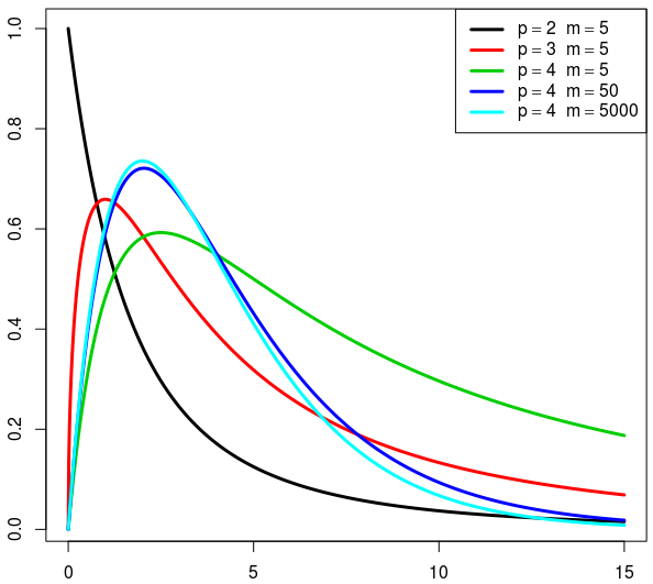
	Probability density function
	Cumulative distribution function
Parameters	p - dimension of the random variables ; m - related to the sample size
Support	if ; otherwise.

In statistics, particularly in hypothesis testing, the Hotelling's T-squared distribution (T²), proposed by Harold Hotelling,^[1] is a multivariate probability distribution that is tightly related to the F-distribution and is most notable for arising as the distribution of a set of sample statistics that are natural generalizations of the statistics underlying the Student's t-distribution. The Hotelling's t-squared statistic (t²) is a generalization of Student's t-statistic that is used in multivariate hypothesis testing.^[2]

Motivation

The distribution arises in multivariate statistics in undertaking tests of the differences between the (multivariate) means of different populations, where tests for univariate problems would make use of a t-test. The distribution is named for Harold Hotelling, who developed it as a generalization of Student's t-distribution.^[1]

Definition

If the vector $d$ is Gaussian multivariate-distributed with zero mean and unit covariance matrix $N(\mathbf {0} _{p},\mathbf {I} _{p,p})$ and $M$ is a $p\times p$ random matrix with a Wishart distribution $W(\mathbf {I} _{p,p},m)$ with unit scale matrix and m degrees of freedom, and d and M are independent of each other, then the quadratic form $X$ has a Hotelling distribution (with parameters $p$ and $m$ ):^[3] $X=md^{T}M^{-1}d\sim T^{2}(p,m).$

It can be shown that if a random variable X has Hotelling's T-squared distribution, $X\sim T_{p,m}^{2}$ , then:^[1] ${\frac {m-p+1}{pm}}X\sim F_{p,m-p+1}$ where $F_{p,m-p+1}$ is the F-distribution with parameters p and m − p + 1.

Hotelling t-squared statistic

Let ${\hat {\mathbf {\Sigma } }}$ be the sample covariance:

${\hat {\mathbf {\Sigma } }}={\frac {1}{n-1}}\sum _{i=1}^{n}\left(\mathbf {x} _{i}-{\overline {\mathbf {x} }}\right)\left(\mathbf {x} _{i}-{\overline {\mathbf {x} }}\right)'$

where we denote transpose by an apostrophe. It can be shown that ${\hat {\mathbf {\Sigma } }}$ is a positive (semi) definite matrix and $(n-1){\hat {\mathbf {\Sigma } }}$ follows a p-variate Wishart distribution with n − 1 degrees of freedom.^[4] The sample covariance matrix of the mean reads ${\hat {\mathbf {\Sigma } }}_{\overline {\mathbf {x} }}={\hat {\mathbf {\Sigma } }}/n$ .^[5]

The Hotelling's t-squared statistic is then defined as:^[6]

$t^{2}=({\overline {\mathbf {x} }}-{\boldsymbol {\mu }})'{\hat {\mathbf {\Sigma } }}_{\overline {\mathbf {x} }}^{-1}({\overline {\mathbf {x} }}-{\boldsymbol {\mathbf {\mu } }})=n({\overline {\mathbf {x} }}-{\boldsymbol {\mu }})'{\hat {\mathbf {\Sigma } }}^{-1}({\overline {\mathbf {x} }}-{\boldsymbol {\mathbf {\mu } }}),$

which is proportional to the Mahalanobis distance between the sample mean and ${\boldsymbol {\mu }}$ . Because of this, one should expect the statistic to assume low values if ${\overline {\mathbf {x} }}\approx {\boldsymbol {\mu }}$ , and high values if they are different.

From the distribution,

$t^{2}\sim T_{p,n-1}^{2}={\frac {p(n-1)}{n-p}}F_{p,n-p},$

where $F_{p,n-p}$ is the F-distribution with parameters p and n − p.

In order to calculate a p-value (unrelated to p variable here), note that the distribution of $t^{2}$ equivalently implies that

${\frac {n-p}{p(n-1)}}t^{2}\sim F_{p,n-p}.$

Then, use the quantity on the left hand side to evaluate the p-value corresponding to the sample, which comes from the F-distribution. A confidence region may also be determined using similar logic.

Motivation

Let ${\mathcal {N}}_{p}({\boldsymbol {\mu }},{\mathbf {\Sigma } })$ denote a p-variate normal distribution with location ${\boldsymbol {\mu }}$ and known covariance ${\mathbf {\Sigma } }$ . Let

${\mathbf {x} }_{1},\dots ,{\mathbf {x} }_{n}\sim {\mathcal {N}}_{p}({\boldsymbol {\mu }},{\mathbf {\Sigma } })$

be n independent identically distributed (iid) random variables, which may be represented as $p\times 1$ column vectors of real numbers. Define

${\overline {\mathbf {x} }}={\frac {\mathbf {x} _{1}+\cdots +\mathbf {x} _{n}}{n}}$

to be the sample mean with covariance ${\mathbf {\Sigma } }_{\overline {\mathbf {x} }}={\mathbf {\Sigma } }/n$ . It can be shown that

$({\overline {\mathbf {x} }}-{\boldsymbol {\mu }})'{\mathbf {\Sigma } }_{\overline {\mathbf {x} }}^{-1}({\overline {\mathbf {x} }}-{\boldsymbol {\mathbf {\mu } }})\sim \chi _{p}^{2},$

where $\chi _{p}^{2}$ is the chi-squared distribution with p degrees of freedom.^[7]

Proof

Proof

Every positive-semidefinite symmetric matrix ${\textstyle {\boldsymbol {M}}}$ has a positive-semidefinite symmetric square root ${\textstyle {\boldsymbol {M}}^{1/2}}$ , and if it is nonsingular, then its inverse has a positive-definite square root ${\textstyle {\boldsymbol {M}}^{-1/2}}$ .

Since ${\textstyle \operatorname {var} \left({\overline {\boldsymbol {x}}}\right)=\mathbf {\Sigma } _{\overline {\mathbf {x} }}}$ , we have ${\begin{aligned}\operatorname {var} \left(\mathbf {\Sigma } _{\overline {\boldsymbol {x}}}^{-1/2}{\overline {\boldsymbol {x}}}\right)&=\mathbf {\Sigma } _{\overline {\boldsymbol {x}}}^{-1/2}{\Big (}\operatorname {var} \left({\overline {\boldsymbol {x}}}\right){\Big )}\left(\mathbf {\Sigma } _{\overline {\boldsymbol {x}}}^{-1/2}\right)^{T}\\[5pt]&=\mathbf {\Sigma } _{\overline {\boldsymbol {x}}}^{-1/2}{\Big (}\operatorname {var} \left({\overline {\boldsymbol {x}}}\right){\Big )}\mathbf {\Sigma } _{\overline {\boldsymbol {x}}}^{-1/2}{\text{ because }}\mathbf {\Sigma } _{\overline {\boldsymbol {x}}}{\text{ is symmetric}}\\[5pt]&=\left(\mathbf {\Sigma } _{\overline {\boldsymbol {x}}}^{-1/2}\mathbf {\Sigma } _{\overline {\boldsymbol {x}}}^{1/2}\right)\left(\mathbf {\Sigma } _{\overline {\boldsymbol {x}}}^{1/2}\mathbf {\Sigma } _{\overline {\boldsymbol {x}}}^{-1/2}\right)\\[5pt]&=\mathbf {I} _{p}.\end{aligned}}$ Consequently $({\overline {\boldsymbol {x}}}-{\boldsymbol {\mu }})^{T}\mathbf {\Sigma } _{\overline {x}}^{-1}({\overline {\boldsymbol {x}}}-{\boldsymbol {\mu }})=\left(\mathbf {\Sigma } _{\overline {x}}^{-1/2}({\overline {\boldsymbol {x}}}-{\boldsymbol {\mu }})\right)^{T}\left(\mathbf {\Sigma } _{\overline {x}}^{-1/2}({\overline {\boldsymbol {x}}}-{\boldsymbol {\mu }})\right)$ and this is simply the sum of squares of ${\textstyle p}$ independent standard normal random variables. Thus its distribution is ${\textstyle \chi _{p}^{2}.}$

Alternatively, one can argue using density functions and characteristic functions, as follows.

Proof

Proof

To show this use the fact that ${\overline {\mathbf {x} }}\sim {\mathcal {N}}_{p}({\boldsymbol {\mu }},{\mathbf {\Sigma } }/n)$ and derive the characteristic function of the random variable $\mathbf {y} =({\bar {\mathbf {x} }}-{\boldsymbol {\mu }})'{\mathbf {\Sigma } }_{\bar {\mathbf {x} }}^{-1}({\bar {\mathbf {x} }}-{\boldsymbol {\mathbf {\mu } }})=({\bar {\mathbf {x} }}-{\boldsymbol {\mu }})'({\mathbf {\Sigma } }/n)^{-1}({\bar {\mathbf {x} }}-{\boldsymbol {\mathbf {\mu } }})$ . As usual, let $|\cdot |$ denote the determinant of the argument, as in $|{\boldsymbol {\Sigma }}|$ .

By definition of characteristic function, we have:^[8] ${\begin{aligned}\varphi _{\mathbf {y} }(\theta )&=\operatorname {E} e^{i\theta \mathbf {y} },\\[5pt]&=\operatorname {E} e^{i\theta ({\overline {\mathbf {x} }}-{\boldsymbol {\mu }})'({\mathbf {\Sigma } }/n)^{-1}({\overline {\mathbf {x} }}-{\boldsymbol {\mathbf {\mu } }})}\\[5pt]&=\int e^{i\theta ({\overline {\mathbf {x} }}-{\boldsymbol {\mu }})'n{\mathbf {\Sigma } }^{-1}({\overline {\mathbf {x} }}-{\boldsymbol {\mathbf {\mu } }})}(2\pi )^{-p/2}|{\boldsymbol {\Sigma }}/n|^{-1/2}\,e^{-(1/2)({\overline {\mathbf {x} }}-{\boldsymbol {\mu }})'n{\boldsymbol {\Sigma }}^{-1}({\overline {\mathbf {x} }}-{\boldsymbol {\mu }})}\,dx_{1}\cdots dx_{p}\end{aligned}}$ There are two exponentials inside the integral, so by multiplying the exponentials we add the exponents together, obtaining: ${\begin{aligned}&=\int (2\pi )^{-p/2}|{\boldsymbol {\Sigma }}/n|^{-1/2}\,e^{-(1/2)({\overline {\mathbf {x} }}-{\boldsymbol {\mu }})'n({\boldsymbol {\Sigma }}^{-1}-2i\theta {\boldsymbol {\Sigma }}^{-1})({\overline {\mathbf {x} }}-{\boldsymbol {\mu }})}\,dx_{1}\cdots dx_{p}\end{aligned}}$ Now take the term $|{\boldsymbol {\Sigma }}/n|^{-1/2}$ off the integral, and multiply everything by an identity $I=|({\boldsymbol {\Sigma }}^{-1}-2i\theta {\boldsymbol {\Sigma }}^{-1})^{-1}/n|^{1/2}\;\cdot \;|({\boldsymbol {\Sigma }}^{-1}-2i\theta {\boldsymbol {\Sigma }}^{-1})^{-1}/n|^{-1/2}$ , bringing one of them inside the integral: ${\begin{aligned}&=|({\boldsymbol {\Sigma }}^{-1}-2i\theta {\boldsymbol {\Sigma }}^{-1})^{-1}/n|^{1/2}|{\boldsymbol {\Sigma }}/n|^{-1/2}\int (2\pi )^{-p/2}|({\boldsymbol {\Sigma }}^{-1}-2i\theta {\boldsymbol {\Sigma }}^{-1})^{-1}/n|^{-1/2}\,e^{-(1/2)n({\overline {\mathbf {x} }}-{\boldsymbol {\mu }})'({\boldsymbol {\Sigma }}^{-1}-2i\theta {\boldsymbol {\Sigma }}^{-1})({\overline {\mathbf {x} }}-{\boldsymbol {\mu }})}\,dx_{1}\cdots dx_{p}\end{aligned}}$ But the term inside the integral is precisely the probability density function of a multivariate normal distribution with covariance matrix $({\boldsymbol {\Sigma }}^{-1}-2i\theta {\boldsymbol {\Sigma }}^{-1})^{-1}/n=\left[n({\boldsymbol {\Sigma }}^{-1}-2i\theta {\boldsymbol {\Sigma }}^{-1})\right]^{-1}$ and mean $\mu$ , so when integrating over all $x_{1},\dots ,x_{p}$ , it must yield $1$ per the probability axioms.^{[clarification needed]} We thus end up with: ${\begin{aligned}&=\left|({\boldsymbol {\Sigma }}^{-1}-2i\theta {\boldsymbol {\Sigma }}^{-1})^{-1}\cdot {\frac {1}{n}}\right|^{1/2}|{\boldsymbol {\Sigma }}/n|^{-1/2}\\&=\left|({\boldsymbol {\Sigma }}^{-1}-2i\theta {\boldsymbol {\Sigma }}^{-1})^{-1}\cdot {\frac {1}{\cancel {n}}}\cdot {\cancel {n}}\cdot {\boldsymbol {\Sigma }}^{-1}\right|^{1/2}\\&=\left|\left[({\cancel {{\boldsymbol {\Sigma }}^{-1}}}-2i\theta {\cancel {{\boldsymbol {\Sigma }}^{-1}}}){\cancel {\boldsymbol {\Sigma }}}\right]^{-1}\right|^{1/2}\\&=|\mathbf {I} _{p}-2i\theta \mathbf {I} _{p}|^{-1/2}\end{aligned}}$ where $I_{p}$ is an identity matrix of dimension $p$ . Finally, calculating the determinant, we obtain: ${\begin{aligned}&=(1-2i\theta )^{-p/2}\end{aligned}}$ which is the characteristic function for a chi-square distribution with $p$ degrees of freedom. $\;\;\;\blacksquare$

Two-sample statistic

If ${\mathbf {x} }_{1},\dots ,{\mathbf {x} }_{n_{x}}\sim N_{p}({\boldsymbol {\mu }},{\mathbf {\Sigma } })$ and ${\mathbf {y} }_{1},\dots ,{\mathbf {y} }_{n_{y}}\sim N_{p}({\boldsymbol {\mu }},{\mathbf {\Sigma } })$ , with the samples independently drawn from two independent multivariate normal distributions with the same mean and covariance, and we define

${\overline {\mathbf {x} }}={\frac {1}{n_{x}}}\sum _{i=1}^{n_{x}}\mathbf {x} _{i}\qquad {\overline {\mathbf {y} }}={\frac {1}{n_{y}}}\sum _{i=1}^{n_{y}}\mathbf {y} _{i}$

as the sample means, and

${\begin{aligned}{\hat {\mathbf {\Sigma } }}_{\mathbf {x} }&={\frac {1}{n_{x}-1}}\sum _{i=1}^{n_{x}}\left(\mathbf {x} _{i}-{\overline {\mathbf {x} }}\right)\left(\mathbf {x} _{i}-{\overline {\mathbf {x} }}\right)'\\{\hat {\mathbf {\Sigma } }}_{\mathbf {y} }&={\frac {1}{n_{y}-1}}\sum _{i=1}^{n_{y}}\left(\mathbf {y} _{i}-{\overline {\mathbf {y} }}\right)\left(\mathbf {y} _{i}-{\overline {\mathbf {y} }}\right)'\end{aligned}}$

as the respective sample covariance matrices. Then

${\hat {\mathbf {\Sigma } }}={\frac {(n_{x}-1){\hat {\mathbf {\Sigma } }}_{\mathbf {x} }+(n_{y}-1){\hat {\mathbf {\Sigma } }}_{\mathbf {y} }}{n_{x}+n_{y}-2}}$

is the unbiased pooled covariance matrix estimate (an extension of pooled variance).

Finally, the Hotelling's two-sample t-squared statistic is

$t^{2}={\frac {n_{x}n_{y}}{n_{x}+n_{y}}}({\overline {\mathbf {x} }}-{\overline {\mathbf {y} }})'{\hat {\mathbf {\Sigma } }}^{-1}({\overline {\mathbf {x} }}-{\overline {\mathbf {y} }})\sim T^{2}(p,n_{x}+n_{y}-2)$

Related concepts

It can be related to the F-distribution by^[4]

${\frac {n_{x}+n_{y}-p-1}{(n_{x}+n_{y}-2)p}}t^{2}\sim F(p,n_{x}+n_{y}-1-p).$

The non-null distribution of this statistic is the noncentral F-distribution (the ratio of a non-central Chi-squared random variable and an independent central Chi-squared random variable) ${\frac {n_{x}+n_{y}-p-1}{(n_{x}+n_{y}-2)p}}t^{2}\sim F(p,n_{x}+n_{y}-1-p;\delta ),$ with $\delta ={\frac {n_{x}n_{y}}{n_{x}+n_{y}}}{\boldsymbol {d}}'\mathbf {\Sigma } ^{-1}{\boldsymbol {d}},$ where ${\boldsymbol {d}}=\mathbf {{\overline {x}}-{\overline {y}}}$ is the difference vector between the population means.

In the two-variable case, the formula simplifies nicely allowing appreciation of how the correlation, $\rho$ , between the variables affects $t^{2}$ . If we define $d_{1}={\overline {x}}_{1}-{\overline {y}}_{1},\qquad d_{2}={\overline {x}}_{2}-{\overline {y}}_{2}$ and $s_{1}={\sqrt {\Sigma _{11}}}\qquad s_{2}={\sqrt {\Sigma _{22}}}\qquad \rho =\Sigma _{12}/(s_{1}s_{2})=\Sigma _{21}/(s_{1}s_{2})$ then $t^{2}={\frac {n_{x}n_{y}}{(n_{x}+n_{y})(1-\rho ^{2})}}\left[\left({\frac {d_{1}}{s_{1}}}\right)^{2}+\left({\frac {d_{2}}{s_{2}}}\right)^{2}-2\rho \left({\frac {d_{1}}{s_{1}}}\right)\left({\frac {d_{2}}{s_{2}}}\right)\right]$ Thus, if the differences in the two rows of the vector $\mathbf {d} ={\overline {\mathbf {x} }}-{\overline {\mathbf {y} }}$ are of the same sign, in general, $t^{2}$ becomes smaller as $\rho$ becomes more positive. If the differences are of opposite sign $t^{2}$ becomes larger as $\rho$ becomes more positive.

A univariate special case can be found in Welch's t-test.

More robust and powerful tests than Hotelling's two-sample test have been proposed in the literature, see for example the interpoint distance based tests which can be applied also when the number of variables is comparable with, or even larger than, the number of subjects.^[9]^[10]

References

^ ^a ^b ^c Hotelling, H. (1931). "The generalization of Student's ratio". Annals of Mathematical Statistics. 2 (3): 360–378. doi:10.1214/aoms/1177732979.
^ Johnson, R.A.; Wichern, D.W. (2002). Applied multivariate statistical analysis. Vol. 5. Prentice hall.
^ Eric W. Weisstein, MathWorld
^ ^a ^b Mardia, K. V.; Kent, J. T.; Bibby, J. M. (1979). Multivariate Analysis. Academic Press. ISBN 978-0-12-471250-8.
^ Fogelmark, Karl; Lomholt, Michael; Irbäck, Anders; Ambjörnsson, Tobias (3 May 2018). "Fitting a function to time-dependent ensemble averaged data". Scientific Reports. 8 (1): 6984. doi:10.1038/s41598-018-24983-y. PMC 5934400. Retrieved 19 August 2024.
^ "6.5.4.3. Hotelling's T squared".
^ End of chapter 4.2 of Johnson, R.A. & Wichern, D.W. (2002)
^ Billingsley, P. (1995). "26. Characteristic Functions". Probability and measure (3rd ed.). Wiley. ISBN 978-0-471-00710-4.
^ Marozzi, M. (2016). "Multivariate tests based on interpoint distances with application to magnetic resonance imaging". Statistical Methods in Medical Research. 25 (6): 2593–2610. doi:10.1177/0962280214529104. PMID 24740998.
^ Marozzi, M. (2015). "Multivariate multidistance tests for high-dimensional low sample size case-control studies". Statistics in Medicine. 34 (9): 1511–1526. doi:10.1002/sim.6418. PMID 25630579.

External links

Prokhorov, A.V. (2001) [1994], T²-distribution "Hotelling T²-distribution", Encyclopedia of Mathematics, EMS Press

[H1931-1] Hotelling, H. (1931). "The generalization of Student's ratio". Annals of Mathematical Statistics. 2 (3): 360–378. doi:10.1214/aoms/1177732979.

[jonhson-2] Johnson, R.A.; Wichern, D.W. (2002). Applied multivariate statistical analysis. Vol. 5. Prentice hall.

[3] Eric W. Weisstein, MathWorld

[MKB-4] Mardia, K. V.; Kent, J. T.; Bibby, J. M. (1979). Multivariate Analysis. Academic Press. ISBN 978-0-12-471250-8.

[Fogelmark2018-5] Fogelmark, Karl; Lomholt, Michael; Irbäck, Anders; Ambjörnsson, Tobias (3 May 2018). "Fitting a function to time-dependent ensemble averaged data". Scientific Reports. 8 (1): 6984. doi:10.1038/s41598-018-24983-y. PMC 5934400. Retrieved 19 August 2024.

[6] "6.5.4.3. Hotelling's T squared".

[7] End of chapter 4.2 of Johnson, R.A. & Wichern, D.W. (2002)

[8] Billingsley, P. (1995). "26. Characteristic Functions". Probability and measure (3rd ed.). Wiley. ISBN 978-0-471-00710-4.

[9] Marozzi, M. (2016). "Multivariate tests based on interpoint distances with application to magnetic resonance imaging". Statistical Methods in Medical Research. 25 (6): 2593–2610. doi:10.1177/0962280214529104. PMID 24740998.

[10] Marozzi, M. (2015). "Multivariate multidistance tests for high-dimensional low sample size case-control studies". Statistics in Medicine. 34 (9): 1511–1526. doi:10.1002/sim.6418. PMID 25630579.

[1]

[2]

[3]

[4]

[5]

[6]

[7]

[8]

[9]

[10]

History

Media collections

Hotelling's T-squared distribution

Recent from talks

Recent from talks

Contribute something

Contribute something

Media Pages

Timelines

Articles

Notes collections

Notes

Notes

Days in Chronicle

Hotelling's T-squared distribution

Motivation

Definition

Hotelling t-squared statistic

Motivation

Two-sample statistic

Related concepts

See also

References

External links