Hubbry Logo
Poisson's equationPoisson's equationMain
Open search
Poisson's equation
Community hub
Poisson's equation
logo
8 pages, 0 posts
0 subscribers
Be the first to start a discussion here.
Poisson's equation
Poisson's equation
from Wikipedia
Siméon Denis Poisson

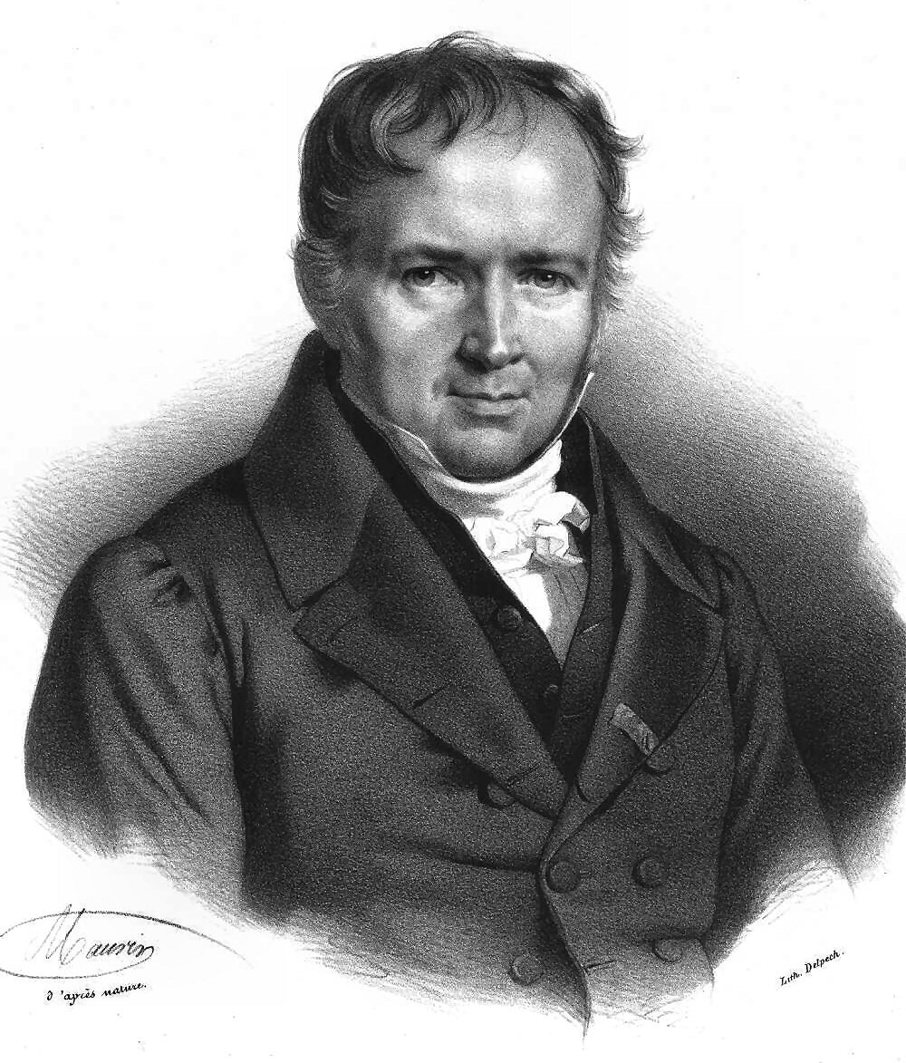
Poisson's equation is an elliptic partial differential equation of broad utility in theoretical physics. For example, the solution to Poisson's equation is the potential field caused by a given electric charge or mass density distribution; with the potential field known, one can then calculate the corresponding electrostatic or gravitational (force) field. It is a generalization of Laplace's equation, which is also frequently seen in physics. The equation is named after French mathematician and physicist Siméon Denis Poisson who published it in 1823.[1][2]

Statement of the equation

[edit]

Poisson's equation is where is the Laplace operator, and and are real or complex-valued functions on a manifold. Usually, is given, and is sought. When the manifold is Euclidean space, the Laplace operator is often denoted as 2, and so Poisson's equation is frequently written as

In three-dimensional Cartesian coordinates, it takes the form

When identically, we obtain Laplace's equation.

Poisson's equation may be solved using a Green's function: where the integral is over all of space. A general exposition of the Green's function for Poisson's equation is given in the article on the screened Poisson equation. There are various methods for numerical solution, such as the relaxation method, an iterative algorithm.

Applications in physics and engineering

[edit]

Newtonian gravity

[edit]

In the case of a gravitational field g due to an attracting massive object of density ρ, Gauss's law for gravity in differential form can be used to obtain the corresponding Poisson equation for gravity. Gauss's law for gravity is

Since the gravitational field is conservative (and irrotational), it can be expressed in terms of a scalar potential ϕ:

Substituting this into Gauss's law, yields Poisson's equation for gravity:

If the mass density is zero, Poisson's equation reduces to Laplace's equation. The corresponding Green's function can be used to calculate the potential at distance r from a central point mass m (i.e., the fundamental solution). In three dimensions the potential is which is equivalent to Newton's law of universal gravitation.

Electrostatics

[edit]

Many problems in electrostatics are governed by the Poisson equation, which relates the electric potential φ to the free charge density , such as those found in conductors.

The mathematical details of Poisson's equation, commonly expressed in SI units (as opposed to Gaussian units), describe how the distribution of free charges generates the electrostatic potential in a given region.

Starting with Gauss's law for electricity (also one of Maxwell's equations) in differential form, one has where is the divergence operator, D is the electric displacement field, and ρf is the free-charge density (describing charges brought from outside).

Assuming the medium is linear, isotropic, and homogeneous (see polarization density), we have the constitutive equation where ε is the permittivity of the medium, and E is the electric field.

Substituting this into Gauss's law and assuming that ε is spatially constant in the region of interest yields In electrostatics, we assume that there is no magnetic field (the argument that follows also holds in the presence of a constant magnetic field).[3] Then, we have that where ∇× is the curl operator. This equation means that we can write the electric field as the gradient of a scalar function φ (called the electric potential), since the curl of any gradient is zero. Thus we can write where the minus sign is introduced so that φ is identified as the electric potential energy per unit charge.[4]

The derivation of Poisson's equation under these circumstances is straightforward. Substituting the potential gradient for the electric field, directly produces Poisson's equation for electrostatics, which is

Specifying the Poisson's equation for the potential requires knowing the charge density distribution. If the charge density is zero, then Laplace's equation results. If the charge density follows a Boltzmann distribution, then the Poisson–Boltzmann equation results. The Poisson–Boltzmann equation plays a role in the development of the Debye–Hückel theory of dilute electrolyte solutions.

Using a Green's function, the potential at distance r from a central point charge Q (i.e., the fundamental solution) is which is Coulomb's law of electrostatics. (For historical reasons, and unlike gravity's model above, the factor appears here and not in Gauss's law.)

The above discussion assumes that the magnetic field is not varying in time. The same Poisson equation arises even if it does vary in time, as long as the Coulomb gauge is used. In this more general class of cases, computing φ is no longer sufficient to calculate E, since E also depends on the magnetic vector potential A, which must be independently computed. See Maxwell's equation in potential formulation for more on φ and A in Maxwell's equations and how an appropriate Poisson's equation is obtained in this case.

Potential of a Gaussian charge density

[edit]

If there is a static spherically symmetric Gaussian charge density where Q is the total charge, then the solution φ(r) of Poisson's equation is given by where erf(x) is the error function.[5] This solution can be checked explicitly by evaluating 2φ.

Note that for r much greater than σ, approaches unity,[6] and the potential φ(r) approaches the point-charge potential, as one would expect. Furthermore, the error function approaches 1 extremely quickly as its argument increases; in practice, for r > 3σ the relative error is smaller than one part in a thousand.[6]

Surface reconstruction

[edit]

Surface reconstruction is an inverse problem. The goal is to digitally reconstruct a smooth surface based on a large number of points pi (a point cloud) where each point also carries an estimate of the local surface normal ni.[7] Poisson's equation can be utilized to solve this problem with a technique called Poisson surface reconstruction.[8]

The goal of this technique is to reconstruct an implicit function f whose value is zero at the points pi and whose gradient at the points pi equals the normal vectors ni. The set of (pi, ni) is thus modeled as a continuous vector field V. The implicit function f is found by integrating the vector field V. Since not every vector field is the gradient of a function, the problem may or may not have a solution: the necessary and sufficient condition for a smooth vector field V to be the gradient of a function f is that the curl of V must be identically zero. In case this condition is difficult to impose, it is still possible to perform a least-squares fit to minimize the difference between V and the gradient of f.

In order to effectively apply Poisson's equation to the problem of surface reconstruction, it is necessary to find a good discretization of the vector field V. The basic approach is to bound the data with a finite-difference grid. For a function valued at the nodes of such a grid, its gradient can be represented as valued on staggered grids, i.e. on grids whose nodes lie in between the nodes of the original grid. It is convenient to define three staggered grids, each shifted in one and only one direction corresponding to the components of the normal data. On each staggered grid we perform trilinear interpolation on the set of points. The interpolation weights are then used to distribute the magnitude of the associated component of ni onto the nodes of the particular staggered grid cell containing pi. Kazhdan and coauthors give a more accurate method of discretization using an adaptive finite-difference grid, i.e. the cells of the grid are smaller (the grid is more finely divided) where there are more data points.[8] They suggest implementing this technique with an adaptive octree.

Fluid dynamics

[edit]

For the incompressible Navier–Stokes equations, given by

The equation for the pressure field is an example of a nonlinear Poisson equation: Notice that the above trace is not sign-definite.

Thermodynamics

[edit]

Thermal conduction is modelled via the Heat equation. Stationary state heat conduction with a source term is modelled via the following Poisson equation:

where is the temperature, is the heat source term and is Thermal conductivity.

See also

[edit]

References

[edit]

Further reading

[edit]
[edit]
Revisions and contributorsEdit on WikipediaRead on Wikipedia
from Grokipedia
Poisson's equation is a second-order linear of elliptic type, generally expressed in three dimensions as 2ϕ(r)=f(r)\nabla^2 \phi(\mathbf{r}) = f(\mathbf{r}), where 2\nabla^2 denotes the Laplacian operator, ϕ\phi is an unknown function, and ff represents a given source term that drives the behavior of the potential. This equation serves as a cornerstone in the mathematical modeling of physical phenomena involving potentials, generalizing 2ϕ=0\nabla^2 \phi = 0, which applies in source-free regions. Named after the French mathematician and physicist , the equation was first published by him in in the Bulletin de la Société Philomatique, where he derived it in the context of electrostatic theory as a relation between and . In physics, Poisson's equation finds extensive applications across multiple domains, most notably in , where it takes the form 2ϕ=ρ/ϵ0\nabla^2 \phi = -\rho / \epsilon_0; here, ϕ\phi is the , ρ\rho is the , and ϵ0\epsilon_0 is the . Similarly, in Newtonian gravitation, the equation describes the Φ\Phi generated by a mass density ρ\rho via 2Φ=4πGρ\nabla^2 \Phi = 4\pi G \rho, with GG being the , linking the potential to the distribution of mass in and . Beyond these, it models steady-state heat conduction with internal heat sources (where ff relates to heat generation), for incompressible flows via the pressure Poisson equation. Mathematically, Poisson's equation is well-posed under appropriate boundary conditions, such as Dirichlet (prescribed potential on the boundary) or (prescribed normal derivative), ensuring unique solutions in bounded domains, and it admits representations for explicit integral solutions in free space. Its elliptic nature implies smooth solutions away from singularities in ff, and numerical methods like finite differences or finite elements are commonly employed for complex geometries due to the lack of closed-form solutions in general cases. Poisson's foundational role extends to broader , influencing developments in and the study of elliptic partial differential equations.

Mathematical foundations

General statement

Poisson's equation is a fundamental in , expressed in its general scalar form as 2ϕ=f,\nabla^2 \phi = f, where ϕ\phi is the function to be determined, 2\nabla^2 denotes the Laplacian operator, and ff is a given source term representing inhomogeneities in the domain. This equation arises in various boundary value problems over a domain ΩRn\Omega \subset \mathbb{R}^n, typically supplemented by appropriate conditions on the boundary Ω\partial \Omega. Poisson's equation reduces to when the source term vanishes (f=0f = 0). The Laplacian operator 2\nabla^2 takes different explicit forms depending on the used. In Cartesian coordinates (x,y,z)(x, y, z), it is given by 2ϕ=2ϕx2+2ϕy2+2ϕz2.\nabla^2 \phi = \frac{\partial^2 \phi}{\partial x^2} + \frac{\partial^2 \phi}{\partial y^2} + \frac{\partial^2 \phi}{\partial z^2}. In spherical coordinates (r,θ,ϕ)(r, \theta, \phi), the expression becomes 2ϕ=1r2r(r2ϕr)+1r2sinθθ(sinθϕθ)+1r2sin2θ2ϕϕ2.\nabla^2 \phi = \frac{1}{r^2} \frac{\partial}{\partial r} \left( r^2 \frac{\partial \phi}{\partial r} \right) + \frac{1}{r^2 \sin \theta} \frac{\partial}{\partial \theta} \left( \sin \theta \frac{\partial \phi}{\partial \theta} \right) + \frac{1}{r^2 \sin^2 \theta} \frac{\partial^2 \phi}{\partial \phi^2}. In cylindrical coordinates (ρ,φ,z)(\rho, \varphi, z), it is 2ϕ=1ρρ(ρϕρ)+1ρ22ϕφ2+2ϕz2.\nabla^2 \phi = \frac{1}{\rho} \frac{\partial}{\partial \rho} \left( \rho \frac{\partial \phi}{\partial \rho} \right) + \frac{1}{\rho^2} \frac{\partial^2 \phi}{\partial \varphi^2} + \frac{\partial^2 \phi}{\partial z^2}. These coordinate-specific forms facilitate solutions in domains with corresponding symmetries. To ensure well-posedness, Poisson's equation is typically paired with boundary conditions on Ω\partial \Omega. The specifies the value of the potential directly: ϕ=g\phi = g on Ω\partial \Omega, where gg is a prescribed function. The , in contrast, specifies the normal derivative: ϕn=h\frac{\partial \phi}{\partial n} = h on Ω\partial \Omega, where n\mathbf{n} is the outward unit normal vector and hh is prescribed. Mixed boundary conditions combining both types may also be employed over different portions of the boundary.

Relation to Laplace's equation

Poisson's equation, in its general form 2ϕ=f\nabla^2 \phi = f, reduces to 2ϕ=0\nabla^2 \phi = 0 in the homogeneous case where the source term f=0f = 0, representing scenarios devoid of distributed sources or charges. This limiting case is fundamental in , where governs the behavior of functions in source-free domains. Physically, Laplace's equation describes equilibrium states in regions without internal sources, such as the electric potential inside a charge-free cavity within a conductor, whereas Poisson's equation accounts for the influence of localized sources, like charge distributions, that drive deviations from harmonicity. This distinction underscores Poisson's equation as a generalization, incorporating inhomogeneities that Laplace's equation idealizes away. Uniqueness theorems for solutions to both equations rely on boundary conditions. Under Dirichlet conditions, where the potential ϕ\phi is specified on the boundary, solutions to Poisson's equation are unique; the difference between any two solutions satisfies Laplace's equation with homogeneous Dirichlet data, which admits only the trivial solution by the maximum principle. For Neumann conditions, specifying the normal derivative ϕ/n\partial \phi / \partial n, uniqueness holds up to an additive constant (a harmonic function), with proofs invoking energy methods or integration by parts to show that non-trivial solutions would contradict boundary compatibility. In both cases, the homogeneous limit ensures that Laplace's solutions are a subset, uniquely determined within the same framework when f=0f = 0. Green's identities provide a mathematical bridge between the equations, facilitating proofs of uniqueness and representation formulas. Green's second identity states that for sufficiently smooth functions ϕ\phi and ψ\psi, V(ϕ2ψψ2ϕ)dV=V(ϕψnψϕn)dS,\int_V (\phi \nabla^2 \psi - \psi \nabla^2 \phi) \, dV = \int_{\partial V} \left( \phi \frac{\partial \psi}{\partial n} - \psi \frac{\partial \phi}{\partial n} \right) dS, where VV is a volume with boundary V\partial V and /n\partial / \partial n denotes the outward normal derivative. When ψ\psi satisfies (2ψ=0\nabla^2 \psi = 0) and ϕ\phi satisfies Poisson's (2ϕ=f\nabla^2 \phi = f), the identity simplifies to VϕfdV=V(ϕψnψϕn)dS\int_V \phi f \, dV = \int_{\partial V} \left( \phi \frac{\partial \psi}{\partial n} - \psi \frac{\partial \phi}{\partial n} \right) dS, linking source integrals to boundary data and highlighting how functions (ψ\psi) can represent solutions to the inhomogeneous problem. This relation is pivotal in deriving via Green's functions, where the fundamental solution to is adjusted for the source term in Poisson's.

Derivations and theoretical context

From Gauss's law

Poisson's equation arises in physical contexts through the application of Gauss's divergence theorem, which relates the flux of a vector field through a closed surface to the divergence of that field within the enclosed volume. The theorem states that for a vector field F\mathbf{F}, V(F)dV=SFdS,\int_V (\nabla \cdot \mathbf{F}) \, dV = \oint_S \mathbf{F} \cdot d\mathbf{S}, where VV is the volume and SS its bounding surface. This integral form allows derivation of differential equations from physical laws expressed as surface integrals. In electrostatics and gravitation, the integral forms of Gauss's law quantify the total "source" (charge or mass) enclosed by a surface, and applying the divergence theorem yields the local differential relation between the field and its source density. In , in integral form asserts that the through a closed surface equals the enclosed charge divided by the ϵ0\epsilon_0, SEdS=Qenclϵ0.\oint_S \mathbf{E} \cdot d\mathbf{S} = \frac{Q_{\text{encl}}}{\epsilon_0}. The ϵ0\epsilon_0, with value 8.854×10¹²F m18.854 \times 10^{-12} \, \text{F m}^{-1}, measures the electric field's strength in for a given . Applying the gives the differential form E=ρ/ϵ0\nabla \cdot \mathbf{E} = \rho / \epsilon_0, where ρ\rho is the . Defining the ϕ\phi such that E=ϕ\mathbf{E} = -\nabla \phi, substitution yields (ϕ)=ρϵ0    2ϕ=ρϵ0.\nabla \cdot (-\nabla \phi) = \frac{\rho}{\epsilon_0} \implies \nabla^2 \phi = -\frac{\rho}{\epsilon_0}. This is Poisson's equation for electrostatics. The gravitational analog follows similarly. Gauss's law for gravity in integral form states that the flux of the gravitational field g\mathbf{g} through a closed surface equals 4πG-4\pi G times the enclosed mass, SgdS=4πGMencl,\oint_S \mathbf{g} \cdot d\mathbf{S} = -4\pi G M_{\text{encl}}, where GG is the gravitational constant, with value 6.674×10¹¹m3kg1s26.674 \times 10^{-11} \, \text{m}^3 \text{kg}^{-1} \text{s}^{-2}, quantifying the strength of gravitational attraction between masses. The divergence theorem produces the differential form g=4πGρ\nabla \cdot \mathbf{g} = -4\pi G \rho, with ρ\rho now the mass density. The gravitational potential Φ\Phi is defined by g=Φ\mathbf{g} = -\nabla \Phi, so (Φ)=4πGρ    2Φ=4πGρ.\nabla \cdot (-\nabla \Phi) = -4\pi G \rho \implies \nabla^2 \Phi = 4\pi G \rho. This yields Poisson's equation for Newtonian .

In vector calculus

In , Poisson's equation arises as a fundamental expressing the relationship between a ϕ\phi and a source term ff, in the coordinate-independent form 2ϕ=f\nabla^2 \phi = f, where 2\nabla^2 denotes the Laplacian operator defined abstractly as the divergence of the , 2ϕ=(ϕ)\nabla^2 \phi = \nabla \cdot (\nabla \phi)./04%3A_Line_and_Surface_Integrals/4.06%3A_Gradient_Divergence_Curl_and_Laplacian) This identity holds in any where the ϕ\nabla \phi produces a from the scalar ϕ\phi, and the \nabla \cdot measures the of that field, yielding a scalar second-order operator independent of specific coordinate systems./04%3A_Line_and_Surface_Integrals/4.06%3A_Gradient_Divergence_Curl_and_Laplacian) Green's first identity provides a key integral formulation that connects the Laplacian to boundary behavior, stated as V(ϕ2ψ+ϕψ)dV=SϕψndS\int_V \left( \phi \nabla^2 \psi + \nabla \phi \cdot \nabla \psi \right) dV = \int_S \phi \frac{\partial \psi}{\partial n} dS for scalar fields ϕ\phi and ψ\psi over a volume VV with boundary SS, where /n\partial / \partial n is the outward normal derivative. Specializing to ψ=ϕ\psi = \phi, this becomes V(ϕ2ϕ+ϕ2)dV=SϕϕndS,\int_V \left( \phi \nabla^2 \phi + |\nabla \phi|^2 \right) dV = \int_S \phi \frac{\partial \phi}{\partial n} dS, which establishes variational principles for solutions to Poisson's equation by relating the volume integral of the source to energy-like functionals involving the . Poisson's equation also emerges as the time-independent limit of parabolic or hyperbolic equations, such as the ut=2u+f\frac{\partial u}{\partial t} = \nabla^2 u + f, where setting ut=0\frac{\partial u}{\partial t} = 0 yields 2u=f\nabla^2 u = -f. Similarly, for the wave equation 2ut2=c22u+f\frac{\partial^2 u}{\partial t^2} = c^2 \nabla^2 u + f, the steady-state condition 2ut2=0\frac{\partial^2 u}{\partial t^2} = 0 reduces to 2u=f/c2\nabla^2 u = -f / c^2, highlighting Poisson's role in stationary scenarios without transient dynamics. These derivations underscore the equation's abstract mathematical structure, applicable across vector fields in Rn\mathbb{R}^n.

Solution techniques

Analytical approaches

Analytical approaches to solving Poisson's equation ∇²φ = f rely on exact methods that exploit the linearity and elliptic nature of the operator, providing closed-form expressions or series representations under suitable boundary conditions and domain geometries. These techniques are particularly effective for simple domains or when the source term f admits a convenient representation in the chosen basis. The Green's function method offers a general representation for the solution in unbounded or free space. For the three-dimensional case with the equation ∇²φ = f, the Green's function G(r, r') satisfies ∇²G = δ(r - r'), where δ is the , and the solution is given by φ(r) = ∫ G(r, r') f(r') dV' over the volume V. In three-dimensional free space, assuming the solution vanishes at infinity, the fundamental solution is G(r, r') = -1/(4π |r - r'|). This form arises from the fundamental solution of the Laplacian and ensures the correct singularity at r = r' while satisfying the homogeneous equation elsewhere. For domains with , methods provide an efficient analytical pathway. Applying the to Poisson's equation yields -|k|² φ̂(k) = f̂(k) in the transform domain, where φ̂ and f̂ are the Fourier transforms of φ and f, respectively, and k is the wave vector. Solving for φ̂(k) = -f̂(k) / |k|² (for k ≠ 0). This requires the compatibility condition that the zero-mode Fourier coefficient f̂(0) = 0, ensuring solvability up to an additive constant. Inverting the transform gives the solution φ(r) = (1/(2π)³) ∫ [-f̂(k) / |k|²] e^{i k · r} d³k. This approach is exact for periodic sources and leverages the , making it ideal for translationally invariant problems. Separation of variables is a powerful technique for bounded domains with separable geometries, such as rectangles or spheres, where boundary conditions can be imposed term by term. Assume Dirichlet conditions φ = 0 on the boundary of a rectangular domain 0 < x < a, 0 < y < b. The source f(x,y) is expanded in a double sine series using the eigenfunctions sin(mπx/a) sin(nπy/b), leading to a solution φ(x,y) as a corresponding series ∑∑ A_{mn} sin(mπx/a) sin(nπy/b), where coefficients A_{mn} are determined by projecting f onto the basis and solving the resulting algebraic system from the eigenvalue problem ∇² (eigenfunction) = -λ (eigenfunction), with λ = (mπ/a)² + (nπ/b)². This method reduces the PDE to an infinite system of ODEs, solvable via orthogonality of the eigenfunctions. Similar expansions apply in spherical coordinates using spherical harmonics for radial symmetry. For far-field approximations, particularly in exterior problems or when sources are localized, multipole expansions provide a hierarchical series representation of the solution. In three dimensions, the potential φ(r) for large |r| is expanded as φ(r) = ∑{l=0}^∞ (1/r^{l+1}) ∑{m=-l}^l Q_{lm} Y_{lm}(θ, ϕ), where Y_{lm} are spherical harmonics, and Q_{lm} are multipole moments computed from integrals involving f(r') and powers of r'. This series converges rapidly far from the sources, offering an asymptotic solution that captures the leading-order behavior, such as monopole, dipole, and higher terms, without solving the full equation globally.

Numerical methods

Numerical methods are essential for solving Poisson's equation in complex geometries or with irregular boundary conditions where analytical solutions are impractical. These approaches discretize the continuous problem into a system of algebraic equations, which can then be solved iteratively or directly, balancing accuracy, computational efficiency, and scalability for large-scale problems. Common techniques leverage structured grids, variational principles, or hierarchical structures to approximate the Laplacian operator and handle the resulting linear systems. Finite difference methods approximate the derivatives in Poisson's equation using discrete differences on a uniform grid. For a two-dimensional case, the Laplacian is approximated by central differences as 2ϕi,jϕi+1,j2ϕi,j+ϕi1,jh2+ϕi,j+12ϕi,j+ϕi,j1h2,\nabla^2 \phi_{i,j} \approx \frac{\phi_{i+1,j} - 2\phi_{i,j} + \phi_{i-1,j}}{h^2} + \frac{\phi_{i,j+1} - 2\phi_{i,j} + \phi_{i,j-1}}{h^2}, where hh is the grid spacing and ϕi,j\phi_{i,j} denotes the solution at grid point (i,j)(i,j). This leads to a sparse linear system that is typically solved using iterative methods due to its size. The Gauss-Seidel method, an iterative relaxation technique, updates each grid point sequentially by solving for ϕi,j\phi_{i,j} using the most recent values of neighboring points, promoting faster convergence than Jacobi iteration for elliptic problems like Poisson's equation. These methods are straightforward to implement on rectangular domains but require careful handling of boundaries to maintain second-order accuracy. Finite element methods reformulate Poisson's equation in a weak variational sense, multiplying by a test function ψ\psi and integrating by parts to obtain ΩϕψdV=ΩfψdV\int_\Omega \nabla \phi \cdot \nabla \psi \, dV = \int_\Omega f \psi \, dV for suitable boundary conditions, where Ω\Omega is the domain. The domain is triangulated into elements, and the solution ϕ\phi is approximated as a linear combination of basis functions (e.g., piecewise linear hat functions) over these elements, leading to a stiffness matrix that assembles element-wise contributions. This approach excels in handling irregular geometries and heterogeneous materials by conforming the mesh to the boundary, achieving optimal convergence rates of order hkh^k for polynomials of degree kk. The resulting system is solved via direct or preconditioned iterative solvers, with the method's flexibility making it widely used in engineering simulations. Multigrid methods accelerate convergence for large discretized systems by employing a hierarchy of grids, from coarse to fine resolutions. Smoothing is applied on the fine grid to eliminate high-frequency errors, residuals are transferred to coarser grids for low-frequency correction, and the improved solution is interpolated back to the fine grid. This V-cycle or W-cycle structure reduces the condition number effectively, achieving grid-independent convergence rates near 0.1 per cycle for Poisson problems on structured grids. Introduced in the 1970s, these methods are particularly efficient for elliptic PDEs, enabling linear-time scaling for problems with millions of unknowns by combining geometric coarsening with robust prolongation and restriction operators. Fast Poisson solvers exploit structure in the problem to reduce complexity below O(N2)O(N^2) for NN degrees of freedom. For periodic boundary conditions, the fast Fourier transform (FFT) diagonalizes the discrete Laplacian in spectral space, allowing exact solution in O(NlogN)O(N \log N) time via convolution with the inverse Green's function. This approach, dating to early FFT applications in numerical PDEs, is ideal for uniform domains like periodic boxes in simulations. For non-periodic or N-body-like problems, hierarchical matrices (H-matrices) approximate the dense potential matrix with low-rank blocks organized in a tree structure, enabling O(NlogN)O(N \log N) or near-linear matrix-vector products and factorizations. These techniques, based on multipole expansions, are crucial for high-fidelity computations in electrostatics and gravity.

Applications in physics

Electrostatics

In electrostatics, Poisson's equation describes the relationship between the electric potential and the charge distribution in a region without time-varying magnetic fields. The equation takes the form 2ϕ=ρϵ0,\nabla^2 \phi = -\frac{\rho}{\epsilon_0}, where ϕ\phi is the electric potential, ρ\rho is the charge density, and ϵ0\epsilon_0 is the vacuum permittivity. This equation is derived from E=ρ/ϵ0\nabla \cdot \mathbf{E} = \rho / \epsilon_0 combined with the definition of the electric field E=ϕ\mathbf{E} = -\nabla \phi. The electric field can thus be obtained from the potential as E=ϕ\mathbf{E} = -\nabla \phi, allowing Poisson's equation to serve as the fundamental governing equation for computing both potential and field from known charges. For a point charge qq located at the origin, the solution in free space is the Coulomb potential ϕ(r)=14πϵ0qr,\phi(\mathbf{r}) = \frac{1}{4\pi \epsilon_0} \frac{q}{r}, which satisfies Poisson's equation everywhere except at the origin where ρ=qδ(r)\rho = q \delta(\mathbf{r}), with δ\delta being the Dirac delta function. This form arises from the symmetry and directly follows from integrating Coulomb's law. For a general, localized charge distribution ρ(r)\rho(\mathbf{r}'), the solution to Poisson's equation in infinite space is given by the integral ϕ(r)=14πϵ0ρ(r)rrdV,\phi(\mathbf{r}) = \frac{1}{4\pi \epsilon_0} \int \frac{\rho(\mathbf{r}')}{|\mathbf{r} - \mathbf{r}'|} \, dV', where the integration extends over all space. This Green's function approach exploits the fundamental solution to the Laplacian, 2(1/r)=4πδ(r)\nabla^2 (1/|\mathbf{r}|) = -4\pi \delta(\mathbf{r}). In cases of spherical symmetry, such as a uniformly charged sphere, the integral simplifies using to yield piecewise potentials: constant inside the sphere and 1/r1/r decay outside, matching the point charge form at large distances. Boundary value problems involving conductors require satisfying conditions like ϕ=0\phi = 0 on the conductor surface. The method of images addresses this by replacing the conductor with fictitious image charges that reproduce the correct boundary conditions in the region of interest, thereby solving Poisson's equation indirectly. For instance, a point charge qq at distance dd above an infinite grounded conducting plane at z=0z=0 is equivalent to an image charge q-q at z=dz = -d, yielding ϕ=0\phi = 0 on the plane and the correct potential for z>0z > 0. This technique extends to spherical conductors and other geometries, ensuring uniqueness via the properties of elliptic partial differential equations.

Newtonian gravity

In Newtonian gravity, Poisson's equation relates the gravitational potential ϕ\phi to the mass density ρ\rho through the form 2ϕ=4πGρ,\nabla^2 \phi = 4\pi G \rho, where GG is the . The g\mathbf{g} is then given by g=ϕ\mathbf{g} = -\nabla \phi, describing the attractive force per unit mass arising from the distributed mass. This equation arises as the gravitational analog to the electrostatic case, differing primarily in the universal attractive nature of and the absence of like-charge repulsion. For a point mass MM at the origin, the solution to Poisson's equation in vacuum (where ρ=0\rho = 0 except at the origin) is the familiar ϕ(r)=GMr,\phi(\mathbf{r}) = -\frac{GM}{r}, with r=rr = |\mathbf{r}|, which yields the inverse-square law for the gravitational field g=GMr2r^\mathbf{g} = -\frac{GM}{r^2} \hat{\mathbf{r}}. This potential is obtained by integrating over the Dirac delta function representation of the point mass in the source term. In cases of spherical symmetry, such as for stars or planets modeled as spherically symmetric mass distributions, the potential can be found by solving Poisson's equation radially. For the exterior region (r>Rr > R, where RR is the radius of the distribution), the solution matches that of a point mass at the center, ϕ(r)=GMr\phi(r) = -\frac{GM}{r}, with MM the total mass. Inside the distribution, the potential depends on the enclosed mass up to radius rr, often resulting in a quadratic form for uniform density, ϕ(r)(3R2r2)\phi(r) \propto - (3R^2 - r^2) (up to constants and scaling), ensuring continuity at the boundary and zero field at the center for symmetry. These solutions follow from Gauss's law applied spherically, confirming that exterior fields are unaffected by the detailed internal distribution. Poisson's equation plays a central role in galactic dynamics for modeling self-gravitating systems, where the mass distribution ρ\rho (from stars, gas, and ) generates the potential that governs orbital motion. In such systems, the equation is solved iteratively or numerically to capture the collective gravitational effects, as in the collisionless coupled with Poisson's form, enabling studies of galactic structure and stability.

Applications in engineering and other fields

Fluid dynamics

In , Poisson's equation frequently appears in the formulation of irrotational flows via the ϕ\phi, defined such that the velocity field is v=ϕ\mathbf{v} = \nabla \phi. For steady, incompressible, irrotational flow, the v=0\nabla \cdot \mathbf{v} = 0 yields 2ϕ=0\nabla^2 \phi = 0, a special case of Poisson's equation with zero source term. In compressible flows or scenarios with distributed sources—such as approximations for weak or variations—the equation generalizes to Poisson's form 2ϕ=f\nabla^2 \phi = f, where ff incorporates the source; for instance, in unsteady irrotational flows with small perturbations, an approximation is 2ϕ1ρρt\nabla^2 \phi \approx -\frac{1}{\rho} \frac{\partial \rho}{\partial t}, derived from the ρt+(ρϕ)=0\frac{\partial \rho}{\partial t} + \nabla \cdot (\rho \nabla \phi) = 0 under the assumption of slowly varying ρ\rho. This form allows modeling of flows where irrotationality holds approximately, such as in low-Mach-number or source-driven problems like point vortices or sinks. Key applications of these potential formulations include design and water wave analysis, often solved using boundary integral methods that reduce the domain to surface integrals for efficiency. In design, the Hess-Smith panel method discretizes the surface into panels with constant source and vortex distributions to satisfy the no-penetration boundary condition and , enabling computation of the and pressure distribution for lift prediction in subsonic flows. For water waves, the in linear theory satisfies beneath the free surface, with boundary integral methods (e.g., via ) used to evaluate the potential at control points on the domain boundaries, facilitating simulations of wave-structure interactions like those around offshore platforms. A prominent use of Poisson's equation in (CFD) is the pressure Poisson equation within projection methods for solving the incompressible Navier-Stokes equations, which enforce mass conservation by correcting an intermediate velocity field. In Chorin's fractional-step method, the momentum equations are advanced to obtain a provisional velocity u\mathbf{u}^*, followed by solving 2p=ρΔtu\nabla^2 p = \frac{\rho}{\Delta t} \nabla \cdot \mathbf{u}^* for the pp, where the correction un+1=uΔtρp\mathbf{u}^{n+1} = \mathbf{u}^* - \frac{\Delta t}{\rho} \nabla p ensures un+1=0\nabla \cdot \mathbf{u}^{n+1} = 0. This approach, introduced by Chorin in 1967, was extended to second-order accuracy on staggered grids by Kim and in 1985, becoming a cornerstone for simulating viscous incompressible flows in complex geometries. Numerical solutions typically employ finite differences, multigrid, or fast Fourier transforms for the elliptic pressure solve, linking directly to broader numerical methods for PDEs.

Thermodynamics

In thermodynamics, Poisson's equation governs the steady-state distribution of temperature in systems with internal heat generation. The steady-state heat conduction equation, derived from the conservation of energy under constant thermal properties, takes the form 2T=Q/k\nabla^2 T = -Q / k, where TT is the field, QQ represents the volumetric generation rate (such as from chemical reactions or ), and kk is the material's thermal conductivity. This balances diffusive with localized sources, ensuring no net accumulation of over time. The assumption of implies T/t=0\partial T / \partial t = 0, simplifying the transient to this Poisson form, which is fundamental for analyzing equilibrium temperature profiles in bounded domains with specified boundary conditions. This formulation finds critical application in heat conduction through solids featuring distributed internal sources, notably in design. In reactor elements, fission processes produce volumetric heat QQ that varies spatially due to distributions, necessitating solutions to 2T=Q/k\nabla^2 T = -Q / k to predict gradients and prevent hotspots that could compromise structural or coolant efficiency. Analytical solutions are limited to simple geometries, so numerical methods like finite element analysis are employed to resolve the equation across complex core configurations, informing safety margins and operational limits. For instance, in cylindrical rods, radial allows separation into ordinary differential equations, but full three-dimensional modeling is required for heterogeneous assemblies. In the realm of thermodynamic potentials, Poisson's equation emerges within descriptions of inhomogeneous systems, particularly those involving charged particles or density variations. The Poisson-Nernst-Planck (PNP) equations couple Poisson's equation for the electrostatic potential ϕ\phi, 2ϕ=ρ/ϵ\nabla^2 \phi = -\rho / \epsilon (where ρ\rho is and ϵ\epsilon is ), with transport equations for species densities driven by gradients in μ\mu. Here, the excess chemical potential often follows a Boltzmann form μex=kBTlnρ\mu_\text{ex} = k_B T \ln \rho, linking the Laplacian source term directly to density-dependent functions f(ρ)f(\rho), which capture local inhomogeneities in fluids or electrolytes. This framework models in non-uniform environments, such as near interfaces or under external fields, where spatial variations in μ\mu influence phase stability and diffusion. Seminal developments in PNP theory emphasize steady-state solutions that resolve these coupled effects, providing insights into thermodynamic consistency across scales. Poisson's equation also connects to in , where it simulates dissipative processes far from equilibrium. In models of transport networks or branching structures, solving the Poisson equation with source terms representing energy dissipation maximizes local rates, aligning with Prigogine's principle of minimum near steady states or maximum production in far-from-equilibrium regimes. For example, in optimizing fluid or flow paths, the equation's solutions yield configurations that enhance irreversible generation while minimizing total dissipation, as seen in biological or engineered systems with tree-like architectures. This relation underscores Poisson's role in quantifying thermodynamic irreversibility, where the source term ff embodies fluxes and affinities driving non-equilibrium evolution. In source-free cases, the equation simplifies to 2T=0\nabla^2 T = 0, modeling reversible, uniform conduction without increase.

Surface reconstruction

Poisson surface reconstruction is a technique that formulates the problem of generating a smooth, watertight surface from an oriented as solving Poisson's equation over a volumetric domain. Given a set of points with estimated surface normals, the method constructs an indicator function χ\chi whose level set approximates the underlying surface. The core idea is to solve the Poisson equation 2χ=V\nabla^2 \chi = \nabla \cdot \mathbf{V}, where V\mathbf{V} is a smoothed vector field derived from the input point normals, ensuring that the gradient of χ\chi aligns with the surface orientation. This approach treats reconstruction globally, avoiding local partitioning or blending issues common in other methods. The algorithm begins by estimating oriented normals at each input point, often using on local neighborhoods, followed by orienting them consistently via . To solve the Poisson equation efficiently, the volume is discretized using an adaptive structure, which refines resolution near the points to handle non-uniform sampling while keeping computational costs manageable. The resulting sparse is solved iteratively with a multigrid solver, producing discrete values of χ\chi at nodes. Finally, the at χ=0.5\chi = 0.5 is extracted using an adaptive algorithm, yielding a that is watertight and manifold. This method finds applications in , where it reconstructs detailed models from laser or structured light scans of objects, producing smooth surfaces despite sparse or irregular point distributions. In medical imaging, Poisson reconstruction processes point clouds derived from MRI or CT data to generate accurate 3D models of anatomical structures, such as liver surfaces for surgical planning and navigation. For instance, screened variants of the algorithm have been used to create patient-specific models from sampled point data in orthopedic and soft tissue reconstruction. Compared to explicit reconstruction methods like or alpha shapes, Poisson surface reconstruction offers superior robustness to noise in point positions and normals, as well as non-uniform sampling densities, by implicitly fitting a smooth function that minimizes deviation from the input orientations. It produces high-quality, watertight meshes without requiring post-processing for hole filling or seam alignment, making it particularly effective for real-world scanned data with imperfections.

References

Add your contribution
Related Hubs
User Avatar
No comments yet.