


Community hub
Quadratic equation
View on WikipediaIn mathematics, a quadratic equation (from Latin quadratus 'square') is an equation that can be rearranged in standard form as[1] where the variable represents an unknown number, and a, b, and c represent known numbers, where a ≠ 0. (If a = 0 and b ≠ 0 then the equation is linear, not quadratic.) The numbers a, b, and c are the coefficients of the equation and may be distinguished by respectively calling them, the quadratic coefficient, the linear coefficient and the constant coefficient or free term.[2]


The values of that satisfy the equation are called solutions of the equation, and roots or zeros of the quadratic function on its left-hand side. A quadratic equation has at most two solutions. If there is only one solution, one says that it is a double root. If all the coefficients are real numbers, there are either two real solutions, or a real double root, or two complex solutions that are complex conjugates of each other. A quadratic equation always has two roots, if complex roots are included and a double root is counted for two. A quadratic equation can be factored into an equivalent equation[3] where r and s are the solutions for .

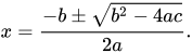
The quadratic formula expresses the solutions in terms of a, b, and c. Completing the square is one of several ways for deriving the formula.
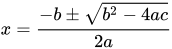
Solutions to problems that can be expressed in terms of quadratic equations were known as early as 2000 BC.[4][5]
The quadratic equation contains only powers of that are non-negative integers, and therefore it is a polynomial equation. In particular, it is a second-degree polynomial equation, since the greatest power is two.
Solving the quadratic equation
[edit]
A quadratic equation whose coefficients are real numbers can have either zero, one, or two distinct real-valued solutions, also called roots. When there is only one distinct root, it can be interpreted as two roots with the same value, called a double root. When there are no real roots, the coefficients can be considered as complex numbers with zero imaginary part, and the quadratic equation still has two complex-valued roots, complex conjugates of each-other with a non-zero imaginary part. A quadratic equation whose coefficients are arbitrary complex numbers always has two complex-valued roots which may or may not be distinct.
The solutions of a quadratic equation can be found by several alternative methods.
Factoring by inspection
[edit]It may be possible to express a quadratic equation ax2 + bx + c = 0 as a product (px + q)(rx + s) = 0. In some cases, it is possible, by simple inspection, to determine values of p, q, r, and s that make the two forms equivalent to one another. If the quadratic equation is written in the second form, then the "Zero Factor Property" states that the quadratic equation is satisfied if px + q = 0 or rx + s = 0. Solving these two linear equations provides the roots of the quadratic.
For most students, factoring by inspection is the first method of solving quadratic equations to which they are exposed.[6]: 202–207 If one is given a quadratic equation in the form x2 + bx + c = 0, the sought factorization has the form (x + q)(x + s), and one has to find two numbers q and s that add up to b and whose product is c (this is sometimes called "Vieta's rule"[7] and is related to Vieta's formulas). As an example, x2 + 5x + 6 factors as (x + 3)(x + 2). The more general case where a does not equal 1 can require a considerable effort in trial and error guess-and-check, assuming that it can be factored at all by inspection.
Except for special cases such as where b = 0 or c = 0, factoring by inspection only works for quadratic equations that have rational roots. This means that the great majority of quadratic equations that arise in practical applications cannot be solved by factoring by inspection.[6]: 207
Completing the square
[edit]
The process of completing the square makes use of the algebraic identity which represents a well-defined algorithm that can be used to solve any quadratic equation.[6]: 207 Starting with a quadratic equation in standard form, ax2 + bx + c = 0

- Divide each side by a, the coefficient of the squared term.
- Subtract the constant term c/a from both sides.
- Add the square of one-half of b/a, the coefficient of x, to both sides. This "completes the square", converting the left side into a perfect square.
- Write the left side as a square and simplify the right side if necessary.
- Produce two linear equations by equating the square root of the left side with the positive and negative square roots of the right side.
- Solve each of the two linear equations.
We illustrate use of this algorithm by solving 2x2 + 4x − 4 = 0


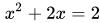

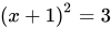
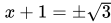
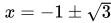
The plus–minus symbol "±" indicates that both and are solutions of the quadratic equation.[8]


Quadratic formula and its derivation
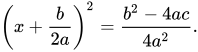
[edit]Completing the square can be used to derive a general formula for solving quadratic equations, called the quadratic formula.[9] The mathematical proof will now be briefly summarized.[10] It can easily be seen, by polynomial expansion, that the following equation is equivalent to the quadratic equation: Taking the square root of both sides, and isolating x, gives:
Some sources, particularly older ones, use alternative parameterizations of the quadratic equation such as ax2 + 2bx + c = 0 or ax2 − 2bx + c = 0 ,[11] where b has a magnitude one half of the more common one, possibly with opposite sign. These result in slightly different forms for the solution, but are otherwise equivalent.
A number of alternative derivations can be found in the literature. These proofs are simpler than the standard completing the square method, represent interesting applications of other frequently used techniques in algebra, or offer insight into other areas of mathematics.
A lesser known quadratic formula, as used in Muller's method, provides the same roots via the equation This can be deduced from the standard quadratic formula by Vieta's formulas, which assert that the product of the roots is c/a. It also follows from dividing the quadratic equation by giving solving this for and then inverting.
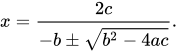



One property of this form is that it yields one valid root when a = 0, while the other root contains division by zero, because when a = 0, the quadratic equation becomes a linear equation, which has one root. By contrast, in this case, the more common formula has a division by zero for one root and an indeterminate form 0/0 for the other root. On the other hand, when c = 0, the more common formula yields two correct roots whereas this form yields the zero root and an indeterminate form 0/0.
When neither a nor c is zero, the equality between the standard quadratic formula and Muller's method, can be verified by cross multiplication, and similarly for the other choice of signs.

Reduced quadratic equation
[edit]It is sometimes convenient to reduce a quadratic equation so that its leading coefficient is one. This is done by dividing both sides by a, which is always possible since a is non-zero. This produces the reduced quadratic equation:[12]

where p = b/a and q = c/a. This monic polynomial equation has the same solutions as the original.
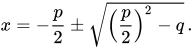
The quadratic formula for the solutions of the reduced quadratic equation, written in terms of its coefficients, is
Discriminant
[edit]
In the quadratic formula, the expression underneath the square root sign is called the discriminant of the quadratic equation, and is often represented using an upper case D or an upper case Greek delta:[13] A quadratic equation with real coefficients can have either one or two distinct real roots, or two distinct complex roots. In this case the discriminant determines the number and nature of the roots. There are three cases:

- If the discriminant is positive, then there are two distinct roots both of which are real numbers. For quadratic equations with rational coefficients, if the discriminant is a square number, then the roots are rational—in other cases they may be quadratic irrationals.
- If the discriminant is zero, then there is exactly one real root sometimes called a repeated or double root or two equal roots.
- If the discriminant is negative, then there are no real roots. Rather, there are two distinct (non-real) complex roots[14] which are complex conjugates of each other. In these expressions i is the imaginary unit.



Thus the roots are distinct if and only if the discriminant is non-zero, and the roots are real if and only if the discriminant is non-negative.
Geometric interpretation
[edit]
The function f(x) = ax2 + bx + c is a quadratic function.[16] The graph of any quadratic function has the same general shape, which is called a parabola. The location and size of the parabola, and how it opens, depend on the values of a, b, and c. If a > 0, the parabola has a minimum point and opens upward. If a < 0, the parabola has a maximum point and opens downward. The extreme point of the parabola, whether minimum or maximum, corresponds to its vertex. The x-coordinate of the vertex will be located at , and the y-coordinate of the vertex may be found by substituting this x-value into the function. The y-intercept is located at the point (0, c).

The solutions of the quadratic equation ax2 + bx + c = 0 correspond to the roots of the function f(x) = ax2 + bx + c, since they are the values of x for which f(x) = 0. If a, b, and c are real numbers and the domain of f is the set of real numbers, then the roots of f are exactly the x-coordinates of the points where the graph touches the x-axis. If the discriminant is positive, the graph touches the x-axis at two points; if zero, the graph touches at one point; and if negative, the graph does not touch the x-axis.
Quadratic factorization
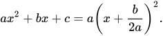
[edit]The term is a factor of the polynomial if and only if r is a root of the quadratic equation It follows from the quadratic formula that In the special case b2 = 4ac where the quadratic has only one distinct root (i.e. the discriminant is zero), the quadratic polynomial can be factored as




Graphical solution
[edit]

The solutions of the quadratic equation may be deduced from the graph of the quadratic function which is a parabola.


If the parabola intersects the x-axis in two points, there are two real roots, which are the x-coordinates of these two points (also called x-intercept).
If the parabola is tangent to the x-axis, there is a double root, which is the x-coordinate of the contact point between the graph and parabola.
If the parabola does not intersect the x-axis, there are two complex conjugate roots. Although these roots cannot be visualized on the graph, their real and imaginary parts can be.[17]
Let h and k be respectively the x-coordinate and the y-coordinate of the vertex of the parabola (that is the point with maximal or minimal y-coordinate. The quadratic function may be rewritten Let d be the distance between the point of y-coordinate 2k on the axis of the parabola, and a point on the parabola with the same y-coordinate (see the figure; there are two such points, which give the same distance, because of the symmetry of the parabola). Then the real part of the roots is h, and their imaginary part are ±d. That is, the roots are or in the case of the example of the figure



Avoiding loss of significance
[edit]Although the quadratic formula provides an exact solution, the result is not exact if real numbers are approximated during the computation, as usual in numerical analysis, where real numbers are approximated by floating point numbers (called "reals" in many programming languages). In this context, the quadratic formula is not completely stable.
This occurs when the roots have different order of magnitude, or, equivalently, when b2 and b2 − 4ac are close in magnitude. In this case, the subtraction of two nearly equal numbers will cause loss of significance or catastrophic cancellation in the smaller root. To avoid this, the root that is smaller in magnitude, r, can be computed as where R is the root that is bigger in magnitude. This is equivalent to using the formula

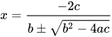
using the plus sign if and the minus sign if


A second form of cancellation can occur between the terms b2 and 4ac of the discriminant, that is when the two roots are very close. This can lead to loss of up to half of correct significant figures in the roots.[11][18]
Examples and applications
[edit]




The golden ratio is found as the positive solution of the quadratic equation

The equations of the circle and the other conic sections—ellipses, parabolas, and hyperbolas—are quadratic equations in two variables.
Given the cosine or sine of an angle, finding the cosine or sine of the angle that is half as large involves solving a quadratic equation.
The process of simplifying expressions involving the square root of an expression involving the square root of another expression involves finding the two solutions of a quadratic equation.
Descartes' theorem states that for every four kissing (mutually tangent) circles, their radii satisfy a particular quadratic equation.
The equation given by Fuss' theorem, giving the relation among the radius of a bicentric quadrilateral's inscribed circle, the radius of its circumscribed circle, and the distance between the centers of those circles, can be expressed as a quadratic equation for which the distance between the two circles' centers in terms of their radii is one of the solutions. The other solution of the same equation in terms of the relevant radii gives the distance between the circumscribed circle's center and the center of the excircle of an ex-tangential quadrilateral.
Critical points of a cubic function and inflection points of a quartic function are found by solving a quadratic equation.
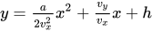
In physics, for motion with constant acceleration , the displacement or position of a moving body can be expressed as a quadratic function of time given the initial position and initial velocity : .


In chemistry, the pH of a solution of weak acid can be calculated from the negative base-10 logarithm of the positive root of a quadratic equation in terms of the acidity constant and the analytical concentration of the acid.
History
[edit]Babylonian mathematicians, as early as 2000 BC (displayed on Old Babylonian clay tablets) could solve problems relating the areas and sides of rectangles. There is evidence dating this algorithm as far back as the Third Dynasty of Ur.[19] In modern notation, the problems typically involved solving a pair of simultaneous equations of the form: which is equivalent to the statement that x and y are the roots of the equation:[20]: 86


The steps given by Babylonian scribes for solving the above rectangle problem, in terms of x and y, were as follows:
- Compute half of p.
- Square the result.
- Subtract q.
- Find the (positive) square root using a table of squares.
- Add together the results of steps (1) and (4) to give x.
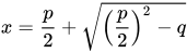
In modern notation this means calculating , which is equivalent to the modern day quadratic formula for the larger real root (if any) with a = 1, b = −p, and c = q.
Geometric methods were used to solve quadratic equations in Babylonia, Egypt, Greece, China, and India. The Egyptian Berlin Papyrus, dating back to the Middle Kingdom (2050 BC to 1650 BC), contains the solution to a two-term quadratic equation.[21] Babylonian mathematicians from circa 400 BC and Chinese mathematicians from circa 200 BC used geometric methods of dissection to solve quadratic equations with positive roots.[22][23] Rules for quadratic equations were given in The Nine Chapters on the Mathematical Art, a Chinese treatise on mathematics.[23][24] These early geometric methods do not appear to have had a general formula. Euclid, the Greek mathematician, produced a more abstract geometrical method around 300 BC. With a purely geometric approach Pythagoras and Euclid created a general procedure to find solutions of the quadratic equation. In his work Arithmetica, the Greek mathematician Diophantus solved the quadratic equation, but giving only one root, even when both roots were positive.[25]
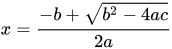
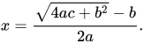
In 628 AD, Brahmagupta, an Indian mathematician, gave in his book Brāhmasphuṭasiddhānta the first explicit (although still not completely general) solution of the quadratic equation ax2 + bx = c as follows: "To the absolute number multiplied by four times the [coefficient of the] square, add the square of the [coefficient of the] middle term; the square root of the same, less the [coefficient of the] middle term, being divided by twice the [coefficient of the] square is the value."[26] This is equivalent to The Bakhshali Manuscript written in India in the 7th century AD contained an algebraic formula for solving quadratic equations, as well as linear indeterminate equations (originally of type ax/c = y).
Muhammad ibn Musa al-Khwarizmi (9th century) developed a set of formulas that worked for positive solutions. Al-Khwarizmi goes further in providing a full solution to the general quadratic equation, accepting one or two numerical answers for every quadratic equation, while providing geometric proofs in the process.[27] He also described the method of completing the square and recognized that the discriminant must be positive,[27][28]: 230 which was proven by his contemporary 'Abd al-Hamīd ibn Turk (Central Asia, 9th century) who gave geometric figures to prove that if the discriminant is negative, a quadratic equation has no solution.[28]: 234 While al-Khwarizmi himself did not accept negative solutions, later Islamic mathematicians that succeeded him accepted negative solutions,[27]: 191 as well as irrational numbers as solutions.[29] Abū Kāmil Shujā ibn Aslam (Egypt, 10th century) in particular was the first to accept irrational numbers (often in the form of a square root, cube root or fourth root) as solutions to quadratic equations or as coefficients in an equation.[30] The 9th century Indian mathematician Sridhara wrote down rules for solving quadratic equations.[31]
The Jewish mathematician Abraham bar Hiyya Ha-Nasi (12th century, Spain) authored the first European book to include the full solution to the general quadratic equation.[32] His solution was largely based on Al-Khwarizmi's work.[27] The writing of the Chinese mathematician Yang Hui (1238–1298 AD) is the first known one in which quadratic equations with negative coefficients of 'x' appear, although he attributes this to the earlier Liu Yi.[33] By 1545 Gerolamo Cardano compiled the works related to the quadratic equations. The quadratic formula covering all cases was first obtained by Simon Stevin in 1594.[34] In 1637 René Descartes published La Géométrie containing the quadratic formula in the form we know today.
Advanced topics
[edit]Alternative methods of root calculation
[edit]Vieta's formulas
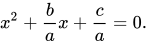
[edit]Vieta's formulas (named after François Viète) are the relations between the roots of a quadratic polynomial and its coefficients. They result from comparing term by term the relation with the equation


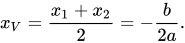
The first Vieta's formula is useful for graphing a quadratic function. Since the graph is symmetric with respect to a vertical line through the vertex, the vertex's x-coordinate is located at the average of the roots (or intercepts). Thus the x-coordinate of the vertex is The y-coordinate can be obtained by substituting the above result into the given quadratic equation, giving Also, these formulas for the vertex can be deduced directly from the formula (see Completing the square)


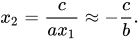
For numerical computation, Vieta's formulas provide a useful method for finding the roots of a quadratic equation in the case where one root is much smaller than the other. If |x2| << |x1|, then x1 + x2 ≈ x1, and we have the estimate: The second Vieta's formula then provides: These formulas are much easier to evaluate than the quadratic formula under the condition of one large and one small root, because the quadratic formula evaluates the small root as the difference of two very nearly equal numbers (the case of large b), which causes round-off error in a numerical evaluation. The figure shows the difference between[clarification needed] (i) a direct evaluation using the quadratic formula (accurate when the roots are near each other in value) and (ii) an evaluation based upon the above approximation of Vieta's formulas (accurate when the roots are widely spaced). As the linear coefficient b increases, initially the quadratic formula is accurate, and the approximate formula improves in accuracy, leading to a smaller difference between the methods as b increases. However, at some point the quadratic formula begins to lose accuracy because of round off error, while the approximate method continues to improve. Consequently, the difference between the methods begins to increase as the quadratic formula becomes worse and worse.

This situation arises commonly in amplifier design, where widely separated roots are desired to ensure a stable operation (see Step response).
Trigonometric solution
[edit]In the days before calculators, people would use mathematical tables—lists of numbers showing the results of calculation with varying arguments—to simplify and speed up computation. Tables of logarithms and trigonometric functions were common in math and science textbooks. Specialized tables were published for applications such as astronomy, celestial navigation and statistics. Methods of numerical approximation existed, called prosthaphaeresis, that offered shortcuts around time-consuming operations such as multiplication and taking powers and roots.[35] Astronomers, especially, were concerned with methods that could speed up the long series of computations involved in celestial mechanics calculations.
It is within this context that we may understand the development of means of solving quadratic equations by the aid of trigonometric substitution. Consider the following alternate form of the quadratic equation,
| 1 |

where the sign of the ± symbol is chosen so that a and c may both be positive. By substituting
| 2 |
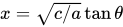
and then multiplying through by cos2(θ) / c, we obtain
| 3 |

Introducing functions of 2θ and rearranging, we obtain
| 4 |
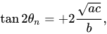
| 5 |
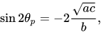
where the subscripts n and p correspond, respectively, to the use of a negative or positive sign in equation [1]. Substituting the two values of θn or θp found from equations [4] or [5] into [2] gives the required roots of [1]. Complex roots occur in the solution based on equation [5] if the absolute value of sin 2θp exceeds unity. The amount of effort involved in solving quadratic equations using this mixed trigonometric and logarithmic table look-up strategy was two-thirds the effort using logarithmic tables alone.[36] Calculating complex roots would require using a different trigonometric form.[37]
To illustrate, let us assume we had available seven-place logarithm and trigonometric tables, and wished to solve the following to six-significant-figure accuracy:

- A seven-place lookup table might have only 100,000 entries, and computing intermediate results to seven places would generally require interpolation between adjacent entries.
- (rounded to six significant figures)







Solution for complex roots in polar coordinates
[edit]If the quadratic equation with real coefficients has two complex roots—the case where requiring a and c to have the same sign as each other—then the solutions for the roots can be expressed in polar form as[38]
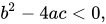

where and

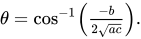
Geometric solution
[edit]
The quadratic equation may be solved geometrically in a number of ways. One way is via Lill's method. The three coefficients a, b, c are drawn with right angles between them as in SA, AB, and BC in Figure 6. A circle is drawn with the start and end point SC as a diameter. If this cuts the middle line AB of the three then the equation has a solution, and the solutions are given by negative of the distance along this line from A divided by the first coefficient a or SA. If a is 1 the coefficients may be read off directly. Thus the solutions in the diagram are −AX1/SA and −AX2/SA.[39]

The Carlyle circle, named after Thomas Carlyle, has the property that the solutions of the quadratic equation are the horizontal coordinates of the intersections of the circle with the horizontal axis.[40] Carlyle circles have been used to develop ruler-and-compass constructions of regular polygons.
Generalization of quadratic equation
[edit]The formula and its derivation remain correct if the coefficients a, b and c are complex numbers, or more generally members of any field whose characteristic is not 2. (In a field of characteristic 2, the element 2a is zero and it is impossible to divide by it.)
The symbol in the formula should be understood as "either of the two elements whose square is b2 − 4ac, if such elements exist". In some fields, some elements have no square roots and some have two; only zero has just one square root, except in fields of characteristic 2. Even if a field does not contain a square root of some number, there is always a quadratic extension field which does, so the quadratic formula will always make sense as a formula in that extension field.

Characteristic 2
[edit]In a field of characteristic 2, the quadratic formula, which relies on 2 being a unit, does not hold. Consider the monic quadratic polynomial over a field of characteristic 2. If b = 0, then the solution reduces to extracting a square root, so the solution is and there is only one root since In summary, See quadratic residue for more information about extracting square roots in finite fields.




In the case that b ≠ 0, there are two distinct roots, but if the polynomial is irreducible, they cannot be expressed in terms of square roots of numbers in the coefficient field. Instead, define the 2-root R(c) of c to be a root of the polynomial x2 + x + c, an element of the splitting field of that polynomial. One verifies that R(c) + 1 is also a root. In terms of the 2-root operation, the two roots of the (non-monic) quadratic ax2 + bx + c are and

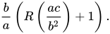
For example, let a denote a multiplicative generator of the group of units of F4, the Galois field of order four (thus a and a + 1 are roots of x2 + x + 1 over F4. Because (a + 1)2 = a, a + 1 is the unique solution of the quadratic equation x2 + a = 0. On the other hand, the polynomial x2 + ax + 1 is irreducible over F4, but it splits over F16, where it has the two roots ab and ab + a, where b is a root of x2 + x + a in F16.
This is a special case of Artin–Schreier theory.
See also
[edit]References
[edit]- ^ Charles P. McKeague (2014). Intermediate Algebra with Trigonometry (reprinted ed.). Academic Press. p. 219. ISBN 978-1-4832-1875-5. Extract of page 219
- ^ Protters & Morrey: "Calculus and Analytic Geometry. First Course".
- ^ The Princeton Review (2020). Princeton Review SAT Prep, 2021: 5 Practice Tests + Review & Techniques + Online Tools. Random House Children's Books. p. 360. ISBN 978-0-525-56974-9. Extract of page 360
- ^ David Mumford; Caroline Series; David Wright (2002). Indra's Pearls: The Vision of Felix Klein (illustrated, reprinted ed.). Cambridge University Press. p. 37. ISBN 978-0-521-35253-6. Extract of page 37
- ^ Mathematics in Action Teachers' Resource Book 4b (illustrated ed.). Nelson Thornes. 1996. p. 26. ISBN 978-0-17-431439-4. Extract of page 26
- ^ a b c Washington, Allyn J. (2000). Basic Technical Mathematics with Calculus, Seventh Edition. Addison Wesley Longman, Inc. ISBN 978-0-201-35666-3.
- ^ Ebbinghaus, Heinz-Dieter; Ewing, John H. (1991), Numbers, Graduate Texts in Mathematics, vol. 123, Springer, p. 77, ISBN 9780387974972.
- ^ Sterling, Mary Jane (2010), Algebra I For Dummies, Wiley Publishing, p. 219, ISBN 978-0-470-55964-2
- ^ Rich, Barnett; Schmidt, Philip (2004), Schaum's Outline of Theory and Problems of Elementary Algebra, The McGraw-Hill Companies, ISBN 978-0-07-141083-0, Chapter 13 §4.4, p. 291
- ^ Himonas, Alex. Calculus for Business and Social Sciences, p. 64 (Richard Dennis Publications, 2001).
- ^ a b Kahan, Willian (November 20, 2004), On the Cost of Floating-Point Computation Without Extra-Precise Arithmetic (PDF), retrieved 2012-12-25
- ^ Alenit͡syn, Aleksandr and Butikov, Evgeniĭ. Concise Handbook of Mathematics and Physics, p. 38 (CRC Press 1997)
- ^ Δ is the initial of the Greek word Διακρίνουσα, Diakrínousa, discriminant.
- ^ Achatz, Thomas; Anderson, John G.; McKenzie, Kathleen (2005). Technical Shop Mathematics. Industrial Press. p. 277. ISBN 978-0-8311-3086-2.
- ^ "Complex Roots Made Visible – Math Fun Facts". Retrieved 1 October 2016.
- ^ Wharton, P. (2006). Essentials of Edexcel Gcse Math/Higher. Lonsdale. p. 63. ISBN 978-1-905-129-78-2.
- ^ Alec Norton, Benjamin Lotto (June 1984), "Complex Roots Made Visible", The College Mathematics Journal, 15 (3): 248–249, doi:10.2307/2686333, JSTOR 2686333
- ^ Higham, Nicholas (2002), Accuracy and Stability of Numerical Algorithms (2nd ed.), SIAM, p. 10, ISBN 978-0-89871-521-7
- ^ Friberg, Jöran (2009). "A Geometric Algorithm with Solutions to Quadratic Equations in a Sumerian Juridical Document from Ur III Umma". Cuneiform Digital Library Journal. 3.
- ^ Stillwell, John (2004). Mathematics and Its History (2nd ed.). Springer. ISBN 978-0-387-95336-6.
- ^ The Cambridge Ancient History Part 2 Early History of the Middle East. Cambridge University Press. 1971. p. 530. ISBN 978-0-521-07791-0.
- ^ Henderson, David W. "Geometric Solutions of Quadratic and Cubic Equations". Mathematics Department, Cornell University. Retrieved 28 April 2013.
- ^ a b Aitken, Wayne. "A Chinese Classic: The Nine Chapters" (PDF). Mathematics Department, California State University. Retrieved 28 April 2013.
- ^ Smith, David Eugene (1958). History of Mathematics. Courier Dover Publications. p. 380. ISBN 978-0-486-20430-7.
{{cite book}}: ISBN / Date incompatibility (help) - ^ Smith, David Eugene (1958). History of Mathematics, Volume 1. Courier Dover Publications. p. 134. ISBN 978-0-486-20429-1.
{{cite book}}: ISBN / Date incompatibility (help) Extract of page 134 - ^ Brāhmasphuṭasiddhānta, Colebrook translation, 1817, page 346; cited by Stillwell, John (2010). Mathematics and Its History (3rd ed.). Undergraduate Texts in Mathematics. Springer. p. 93. doi:10.1007/978-1-4419-6053-5. ISBN 978-0-387-95336-6.
- ^ a b c d Katz, V. J.; Barton, B. (2006). "Stages in the History of Algebra with Implications for Teaching". Educational Studies in Mathematics. 66 (2): 185–201. doi:10.1007/s10649-006-9023-7. S2CID 120363574.
- ^ a b Boyer, Carl B. (1991). Merzbach, Uta C. (ed.). A History of Mathematics. John Wiley & Sons, Inc. ISBN 978-0-471-54397-8.
- ^ O'Connor, John J.; Robertson, Edmund F. (1999), "Arabic mathematics: forgotten brilliance?", MacTutor History of Mathematics Archive, University of St Andrews "Algebra was a unifying theory which allowed rational numbers, irrational numbers, geometrical magnitudes, etc., to all be treated as "algebraic objects"."
- ^ Jacques Sesiano, "Islamic mathematics", p. 148, in Selin, Helaine; D'Ambrosio, Ubiratan, eds. (2000), Mathematics Across Cultures: The History of Non-Western Mathematics, Springer, ISBN 978-1-4020-0260-1
- ^ Smith, David Eugene (1958). History of Mathematics. Courier Dover Publications. p. 280. ISBN 978-0-486-20429-1.
{{cite book}}: ISBN / Date incompatibility (help) - ^ Livio, Mario (2006). The Equation that Couldn't Be Solved. Simon & Schuster. ISBN 978-0743258210.
- ^ Ronan, Colin (1985). The Shorter Science and Civilisation in China. Cambridge University Press. p. 15. ISBN 978-0-521-31536-4.
- ^ Struik, D. J.; Stevin, Simon (1958), The Principal Works of Simon Stevin, Mathematics (PDF), vol. II–B, C. V. Swets & Zeitlinger, p. 470
- ^ Ballew, Pat. "Solving Quadratic Equations — By analytic and graphic methods; Including several methods you may never have seen" (PDF). Archived from the original on 9 April 2011. Retrieved 18 April 2013.
- ^ Seares, F. H. (1945). "Trigonometric Solution of the Quadratic Equation". Publications of the Astronomical Society of the Pacific. 57 (339): 307–309. Bibcode:1945PASP...57..307S. doi:10.1086/125759.
- ^ Aude, H. T. R. (1938). "The Solutions of the Quadratic Equation Obtained by the Aid of the Trigonometry". National Mathematics Magazine. 13 (3): 118–121. doi:10.2307/3028750. JSTOR 3028750.
- ^ Simons, Stuart, "Alternative approach to complex roots of real quadratic equations", Mathematical Gazette 93, March 2009, 91–92.
- ^ Bixby, William Herbert (1879), Graphical Method for finding readily the Real Roots of Numerical Equations of Any Degree, West Point N. Y.
- ^ Weisstein, Eric W. "Carlyle Circle". From MathWorld—A Wolfram Web Resource. Retrieved 21 May 2013.
External links
[edit]
- "Quadratic equation", Encyclopedia of Mathematics, EMS Press, 2001 [1994]
- Weisstein, Eric W. "Quadratic equations". MathWorld.
- 101 uses of a quadratic equation Archived 2007-11-10 at the Wayback Machine
- 101 uses of a quadratic equation: Part II Archived 2007-10-22 at the Wayback Machine

Quadratic equation
View on GrokipediaDefinition and Basic Properties
Standard Form
A quadratic equation is an algebraic equation of the second degree with one unknown variable, expressed in its standard form as $ ax^2 + bx + c = 0 $, where $ a $, $ b $, and $ c $ are real coefficients and $ a \neq 0 $.[11][12] This form represents a polynomial equation where the highest power of the variable $ x $ is 2, distinguishing it from linear (degree 1) or cubic (degree 3) equations.[11] The designation "quadratic" originates from the Latin term quadratus, the past participle of quadrare, meaning "to square," which alludes to the squared term $ x^2 $ central to the equation's structure.[13] The coefficient $ a $ scales the quadratic term and determines the parabola's orientation when graphed, while $ b $ and $ c $ adjust the linear and constant components, respectively.[14] Although the focus for solving quadratic equations remains the standard form, the related quadratic function can be expressed in vertex form as $ y = a(x - h)^2 + k $, where $ (h, k) $ identifies the parabola's vertex, aiding in graphical analysis.[15]Coefficients and Discriminant
In the standard form of a quadratic equation, $ ax^2 + bx + c = 0 $, the coefficients $ a $, $ b $, and $ c $ (with $ a \neq 0 $) play distinct roles in defining the equation's graph as a parabola and its solution properties.[16] The coefficient $ a $ determines the direction and scaling of the parabola: if $ a > 0 $, the parabola opens upward; if $ a < 0 $, it opens downward, reflecting the graph across the x-axis. The magnitude of $ a $ affects the width, with larger $ |a| $ values narrowing the parabola and smaller values widening it.[16] The coefficient $ b $ influences the horizontal position of the parabola by setting the axis of symmetry at $ x = -\frac{b}{2a} $, which locates the vertex and turning point.[16] The constant term $ c $ represents the y-intercept, shifting the parabola vertically so that it crosses the y-axis at $ (0, c) $.[16] A key property derived from these coefficients is the discriminant, defined as $ D = b^2 - 4ac $, which appears under the square root in the quadratic formula and determines the nature of the roots without solving the equation.[17] The value of the discriminant classifies the roots as follows: if $ D > 0 $, there are two distinct real roots, corresponding to the parabola intersecting the x-axis at two points; if $ D = 0 $, there is exactly one real root (repeated), meaning the parabola touches the x-axis at its vertex; if $ D < 0 $, there are two complex conjugate roots, and the parabola does not intersect the x-axis.[17] Additionally, Vieta's formulas connect the coefficients to the roots: for roots $ r_1 $ and $ r_2 $, the sum $ r_1 + r_2 = -\frac{b}{a} $ and the product $ r_1 r_2 = \frac{c}{a} $, providing symmetric relations that highlight the interplay among $ a $, $ b $, and $ c $.[18]Algebraic Solution Methods
Factoring by Inspection
Factoring by inspection is an algebraic technique for solving quadratic equations of the form $ ax^2 + bx + c = 0 $ by expressing the quadratic as a product of two linear factors $ (px + q)(rx + s) = 0 $, where $ pr = a $, $ qs = c $, and $ ps + qr = b $.[19] This method relies on identifying suitable integer or rational factors through trial and error or systematic search, leveraging the zero-factor property to find the roots as $ x = -q/p $ and $ x = -s/r $.[20] When the leading coefficient $ a = 1 $, the process simplifies to finding two numbers that multiply to $ c $ and add to $ b $. For example, in the equation $ x^2 + 5x + 6 = 0 $, the numbers 2 and 3 satisfy $ 2 \times 3 = 6 $ and $ 2 + 3 = 5 $, yielding the factorization $ (x + 2)(x + 3) = 0 $ with roots $ x = -2 $ and $ x = -3 $.[19] For cases where $ a \neq 1 $, the AC method is commonly used: first, identify two numbers that multiply to $ ac $ and add to $ b $, then rewrite the middle term and factor by grouping. Consider $ 2x^2 + 7x + 3 = 0 $; here, $ ac = 6 $, and the numbers 6 and 1 multiply to 6 and add to 7, so rewrite as $ 2x^2 + 6x + x + 3 = 0 $, group as $ (2x^2 + 6x) + (x + 3) = 0 $, factor to $ 2x(x + 3) + 1(x + 3) = 0 $, and obtain $ (2x + 1)(x + 3) = 0 $ with roots $ x = -1/2 $ and $ x = -3 $.[20] A quadratic equation can be factored into linear factors over the real numbers if its discriminant $ b^2 - 4ac $ is positive, indicating two distinct real roots, or zero, indicating a repeated real root.[21] This method works best with integer coefficients and rational roots, as the factors are typically integers in such cases.[19] The primary advantage of factoring by inspection is that it provides exact roots directly without invoking a general formula, making it intuitive for simple polynomials and useful in educational settings as an introductory solving technique.[19] However, it has limitations, particularly with non-integer coefficients, where finding suitable factors becomes trial-intensive or impractical, and it fails entirely for quadratics without rational roots even if real roots exist.[20]Completing the Square
Completing the square is an algebraic technique for solving quadratic equations of the form $ ax^2 + bx + c = 0 $ by rewriting the expression as a difference of a perfect square trinomial and a constant, facilitating the extraction of roots via square roots. This method is particularly useful when the quadratic does not factor easily over the integers and provides insight into the equation's structure by transforming it into a form equivalent to the vertex representation of a parabola.[22] The origins of completing the square trace back to Old Babylonian mathematics around 1800 BCE, where it was employed geometrically to solve quadratic problems, such as completing L-shaped figures into squares on clay tablets like YBC 6967.[5] In the 9th century, the Persian scholar Muhammad ibn Musa al-Khwarizmi systematized the approach in his Compendium on Calculation by Completion and Balancing, presenting it as a core method for three cases of quadratics through geometric constructions, without considering negative roots.[23] Brahmagupta's 7th-century algebraic solutions to quadratics preceded al-Khwarizmi's geometric systematization of completing the square, which together influenced later European developments, such as those by Fibonacci in the 13th century.[5] Geometrically, completing the square can be demonstrated using areas of squares and rectangles. For the equation $ x^2 + bx = c $, construct a square of side length $ x $ to represent the $ x^2 $ term. Attach two rectangles, each with dimensions $ x \times \frac{b}{2} $, to two adjacent sides of the square, and place a square of side $ \frac{b}{2} $ in the corner to complete a larger square with side length $ x + \frac{b}{2} $. The area of this larger square is $ \left(x + \frac{b}{2}\right)^2 = x^2 + bx + \left(\frac{b}{2}\right)^2 = c + \left(\frac{b}{2}\right)^2 $, thus completing the square geometrically and illustrating the connection between algebraic manipulation and geometric areas.[24] To solve a quadratic equation using completing the square, follow these steps for the general form $ ax^2 + bx + c = 0 $, assuming $ a \neq 0 $:- Divide both sides by $ a $ to obtain $ x^2 + \frac{b}{a}x + \frac{c}{a} = 0 $, making the leading coefficient 1.[22]
- Move the constant term to the right side: $ x^2 + \frac{b}{a}x = -\frac{c}{a} $.[22]
- Add $ \left( \frac{b}{2a} \right)^2 $ to both sides to complete the square on the left: $ x^2 + \frac{b}{a}x + \left( \frac{b}{2a} \right)^2 = -\frac{c}{a} + \left( \frac{b}{2a} \right)^2 $. The left side factors as $ \left( x + \frac{b}{2a} \right)^2 $.[22]
- Take the square root of both sides: $ x + \frac{b}{2a} = \pm \sqrt{ -\frac{c}{a} + \left( \frac{b}{2a} \right)^2 } $.[22]
- Solve for $ x $: $ x = -\frac{b}{2a} \pm \sqrt{ \left( \frac{b}{2a} \right)^2 - \frac{c}{a} } $.[22]
Quadratic Formula and Derivation
The quadratic formula provides a universal algebraic method to find the roots of any quadratic equation of the form $ ax^2 + bx + c = 0 $, where $ a \neq 0 $, $ b $, and $ c $ are real coefficients. The solutions, or roots, are given byGeometric and Graphical Solutions
Parabola Interpretation
The graph of a quadratic function $ y = ax^2 + bx + c $, where $ a \neq 0 $, is a parabola.[32] If $ a > 0 $, the parabola opens upward, indicating a minimum value at the vertex; if $ a < 0 $, it opens downward, indicating a maximum value.[33] This U-shaped curve is symmetric and extends infinitely in the direction of its opening.[32] Geometrically, the parabola is defined as the locus of points equidistant from a fixed point (the focus) and a fixed straight line (the directrix). This focus-directrix definition is equivalent to the quadratic equation form in a coordinate system.[34] The vertex of the parabola represents its turning point and can be found using the formulas $ x = -\frac{b}{2a} $ for the x-coordinate and $ y = c - \frac{b^2}{4a} $ for the y-coordinate.[32] The axis of symmetry is the vertical line $ x = -\frac{b}{2a} $, which passes through the vertex and divides the parabola into two mirror-image halves.[33] The y-intercept occurs at the point $ (0, c) $, where the parabola crosses the y-axis.[35] The x-intercepts, or points where the parabola crosses the x-axis, correspond to the real roots of the quadratic equation $ ax^2 + bx + c = 0 $, obtained by setting $ y = 0 $.[32] These intercepts lie symmetrically about the axis of symmetry if two exist, providing visual insight into the number and location of solutions.[33] The standard parabola $ y = x^2 $ serves as the parent function, and the general form arises through transformations: a vertical stretch or compression by $ |a| $, a reflection over the x-axis if $ a < 0 $, a horizontal shift by $ -\frac{b}{2a} $ units, and a vertical shift by $ c $ units.[32] These transformations preserve the parabolic shape while altering its position, orientation, and scale.[33]Geometric Constructions
There is a close connection between geometry and quadratic equations, as many geometric problems naturally lead to quadratic equations, and historically, such equations were solved geometrically using ruler and compass constructions in ancient Greek mathematics. The roots of quadratic equations can be constructed geometrically using a ruler (straightedge) and compass, methods that trace their origins to ancient Greek mathematics and form the basis of Euclidean geometry. These constructions transform the algebraic problem into finding specific lengths on a plane through intersections of lines and circles, where the coefficients are represented as given lengths. In Euclid's Elements, particularly Book II, such techniques are developed through propositions that geometrically interpret completing the square and extracting square roots, allowing solutions to specific quadratic forms without symbolic algebra. For instance, Proposition II.6 provides a construction for equations of the form by erecting a perpendicular of length at the midpoint of a segment of length and drawing a circle of radius centered at one endpoint, with the intersection point yielding a length related to the root via the difference of squares: .[36] Completing the square also has a direct geometric visualization using areas of squares and rectangles for equations like . By constructing a large square of side composed of a central square of side , two rectangles each of area , and a small square of side , the area equality demonstrates the completion: . Quadratic equations frequently arise from geometric intersections, such as between a straight line and a circle. Substituting the equation of the line into the circle's equation produces a quadratic whose solutions correspond to the coordinates of the intersection points. A notable historical example is the construction of the golden ratio, which satisfies the quadratic equation (or ), achieved geometrically in Euclid's Elements, Book VI, Proposition 30.[37] To address the general equation , first reduce it to the monic depressed form by constructing the ratios and . This division is performed using similar triangles: draw a line segment of length , erect a perpendicular of length at one end, and draw a parallel line from a unit length to intersect, yielding as the intercepted segment. The same applies for . With and as lengths, construct perpendiculars to a base line to position coefficients spatially, then draw circles whose radii or diameters incorporate these lengths. Intersections with the base line or other constructed lines provide the root lengths, relying on Euclidean propositions for bisecting segments (Book I, Prop. 10), erecting perpendiculars (Book I, Prop. 11), and circle properties (Book III, Prop. 31).[38] A specific example is the geometric solution for using a circle with a diameter determined by the coefficients, known as the Carlyle circle. Draw a base line and select origin on . Erect a perpendicular to at , marking point at unit distance 1 from . From , along in the negative direction, mark point at distance from . From , erect a perpendicular to in the same direction as if (or opposite if ), marking point at distance from . Construct the circle with diameter : first, find the midpoint of as center using bisection, then set the radius to half with the compass. This circle intersects at two points and (potentially including if a root is zero), where the directed distances from to and are the roots of the equation. The method works because the circle's defining equation, when restricted to the base line, simplifies to the quadratic via the diameter endpoint property and the right-angle theorem in a semicircle (Euclid Book III, Prop. 31). For real roots, the discriminant must be non-negative, ensuring two intersections on ; complex roots do not yield real intersections.[39] These constructions are limited to producing constructible numbers, which are real numbers obtainable from the rationals via a finite tower of quadratic field extensions using the given coefficient lengths as starting points. Roots of quadratics with constructible coefficients are always constructible, as solving involves at most one square root extraction, corresponding to a single quadratic extension. However, this restricts applicability to problems where solutions lie in such fields; for instance, roots requiring cubic or higher odd-degree extensions (as in angle trisection or cube duplication) cannot be constructed solely with ruler and compass, a result formalized in Galois theory.[40]Graphical Methods
Graphical methods for solving quadratic equations involve plotting the quadratic function and identifying the points where the graph intersects the x-axis, which correspond to the real roots of the equation. To apply this approach, one graphs the equation $ y = ax^2 + bx + c $, where $ a $, $ b $, and $ c $ are constants, and the x-intercepts provide the approximate values of the roots by visual inspection or measurement on the graph.[41][42] This method leverages the parabolic shape of the graph, allowing users to visualize the behavior of the quadratic.[43] The vertex of the parabola and its axis of symmetry play key roles in estimating roots more effectively. The vertex represents the turning point, and the axis of symmetry is the vertical line through the vertex, which bisects the parabola; roots, if real, lie symmetric about this axis, enabling quicker approximations of their positions relative to the vertex.[43] For instance, if the vertex is known to be at a certain x-value, one can estimate the roots by considering equal distances on either side where the graph crosses the x-axis. Digital tools enhance the precision of graphical solutions. Interactive graphing calculators like Desmos allow users to plot the quadratic function and zoom in on x-intercepts or use built-in features to detect exact intersection points, bridging the gap between visual approximation and algebraic accuracy.[44] These tools facilitate exploration of how changes in coefficients affect root locations. This method offers advantages in building intuition, as it visually reveals the number of real roots (zero, one, or two) and their approximate locations without complex calculations, making it accessible for initial explorations.[45] However, it has disadvantages in precision, particularly with hand-drawn graphs where scale and resolution limit accuracy, and it cannot directly identify complex roots.[46] As an example, consider sketching $ y = x^2 - 5x + 6 $; the parabola opens upward, and visual estimation of x-intercepts around x=2 and x=3 provides a quick sense of the roots before applying algebraic methods.[47]Numerical and Practical Considerations
Avoiding Loss of Significance
When computing the roots of a quadratic equation $ ax^2 + bx + c = 0 $ using the quadratic formula, numerical instability arises due to catastrophic cancellation in floating-point arithmetic, particularly when $ |b| $ is much larger than $ \sqrt{|4ac|} $, causing the terms $ -b \pm \sqrt{b^2 - 4ac} $ to be nearly equal in magnitude but opposite in sign for one root.[48] This subtraction of closely valued large numbers leads to a severe loss of significant digits, resulting in inaccurate computation of the smaller root in absolute value, while the larger root remains reliable.[49] The issue is exacerbated when the discriminant $ D = b^2 - 4ac $ is small relative to $ b^2 $, as the square root $ \sqrt{D} $ approximates $ |b| $, amplifying roundoff errors in finite-precision systems like IEEE 754 double precision.[50] To mitigate this loss of significance, an alternative formulation computes the problematic root by rationalizing the numerator: for the root nearer to $ -c/b $, use $ x = \frac{2c}{-b - \operatorname{sign}(b) \sqrt{D}} $, where the sign ensures addition rather than subtraction of large terms.[48] The stable root (farther from zero) is calculated first via the standard formula with the sign that avoids cancellation—specifically, $ x_1 = \frac{-b - \operatorname{sign}(b) \sqrt{D}}{2a} $—and the second root $ x_2 $ follows from the rationalized form $ x_2 = \frac{2c}{ -b - \operatorname{sign}(b) \sqrt{D} } $, preserving full precision for both.[51] This approach, originally highlighted by Carl Friedrich Gauss and refined by William Kahan, ensures that the computed roots satisfy Vieta's formulas $ x_1 + x_2 = -b/a $ and $ x_1 x_2 = c/a $ within machine epsilon.[49][50] Consider the equation $ 0.0001x^2 + 100000x + 0.002 = 0 $ in double-precision arithmetic (approximately 15 decimal digits). The exact roots are approximately $ -10^9 $ and $ -2 \times 10^{-8} $. Using the standard formula for the smaller root yields $ x \approx 0 $ due to cancellation in $ -b + \sqrt{D} \approx -4 \times 10^{-12} $, losing all precision beyond the first few digits.[49] Applying the rationalized form gives $ x \approx -2 \times 10^{-8} $, accurate to nearly full precision, while the larger root remains stable in both methods.[48] For software implementations, normalize the equation to reduced (monic) form by dividing coefficients by $ a $ before applying the stable algorithm, which scales the problem to unit leading coefficient and reduces overflow risks.[51] Additionally, compute the discriminant with extra precision—such as Kahan's method of representing $ b^2 $ and $ 4ac $ as sums of high- and low-order parts to avoid underflow in $ D $—ensuring robustness across floating-point environments like MATLAB or C++.[50] Many numerical libraries incorporate these techniques to guarantee backward stability.[51]Reduced Form and Vieta's Formulas
The reduced form of a quadratic equation, also known as the monic form, is obtained by dividing the general equation (with ) by the leading coefficient , yielding , where and .[52] This normalization simplifies the expression by setting the coefficient of to 1, facilitating comparisons and substitutions without altering the roots.[52] Vieta's formulas, named after the French mathematician François Viète (1540–1603), establish relationships between the coefficients of a polynomial and the sums and products of its roots.[53] For the general quadratic equation with roots and , the sum of the roots is and the product is .[18] In the reduced form , these relations simplify to and .[18] These formulas arise from expanding the factored representation of the equation.[18] Assuming roots and , the monic quadratic can be written as , which expands to- For the equation , the sum of the roots is and the product is .
- The equation has roots and , with sum and product .
- The quadratic equation with roots and is .
- For the quadratic polynomial , if and are the roots, then .[54]