Recent from talks
Contribute something
Nothing was collected or created yet.
Sine and cosine
View on Wikipedia| Sine and cosine | |
|---|---|
| General information | |
| General definition | |
| Fields of application | Trigonometry, Fourier series, etc. |
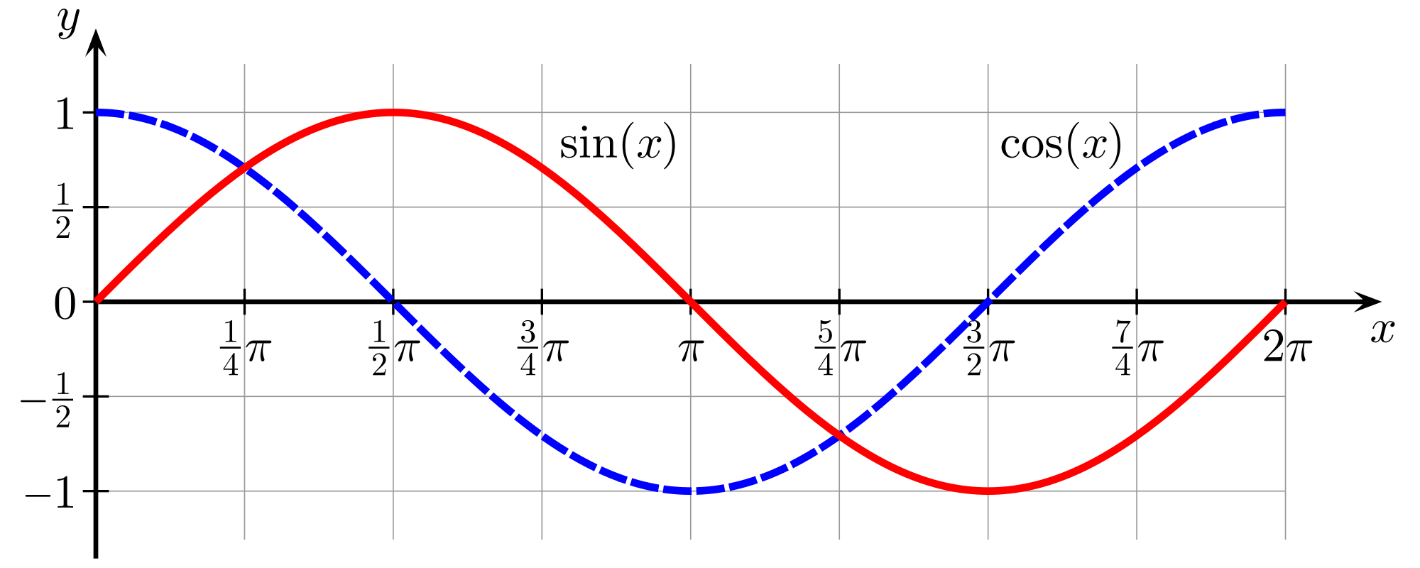
In mathematics, sine and cosine are trigonometric functions of an angle. The sine and cosine of an acute angle are defined in the context of a right triangle: for the specified angle, its sine is the ratio of the length of the side opposite that angle to the length of the longest side of the triangle (the hypotenuse), and the cosine is the ratio of the length of the adjacent leg to that of the hypotenuse. For an angle , the sine and cosine functions are denoted as and .
The definitions of sine and cosine have been extended to any real value in terms of the lengths of certain line segments in a unit circle. More modern definitions express the sine and cosine as infinite series, or as the solutions of certain differential equations, allowing their extension to arbitrary positive and negative values and even to complex numbers.
The sine and cosine functions are commonly used to model periodic phenomena such as sound and light waves, the position and velocity of harmonic oscillators, sunlight intensity and day length, and average temperature variations throughout the year. They can be traced to the jyā and koṭi-jyā functions used in Indian astronomy during the Gupta period.
Elementary descriptions
[edit]Right-angled triangle definition
[edit]
To define the sine and cosine of an acute angle , start with a right triangle that contains an angle of measure ; in the accompanying figure, angle in a right triangle is the angle of interest. The three sides of the triangle are named as follows:[1]
- The opposite side is the side opposite to the angle of interest; in this case, it is .
- The hypotenuse is the side opposite the right angle; in this case, it is . The hypotenuse is always the longest side of a right-angled triangle.
- The adjacent side is the remaining side; in this case, it is . It forms a side of (and is adjacent to) both the angle of interest and the right angle.
Once such a triangle is chosen, the sine of the angle is equal to the length of the opposite side divided by the length of the hypotenuse, and the cosine of the angle is equal to the length of the adjacent side divided by the length of the hypotenuse:[1]
The other trigonometric functions of the angle can be defined similarly; for example, the tangent is the ratio between the opposite and adjacent sides or equivalently the ratio between the sine and cosine functions. The reciprocal of sine is cosecant, which gives the ratio of the hypotenuse length to the length of the opposite side. Similarly, the reciprocal of cosine is secant, which gives the ratio of the hypotenuse length to that of the adjacent side. The cotangent function is the ratio between the adjacent and opposite sides, a reciprocal of a tangent function. These functions can be formulated as:[1]
Special angle measures
[edit]As stated, the values and appear to depend on the choice of a right triangle containing an angle of measure . However, this is not the case as all such triangles are similar, and so the ratios are the same for each of them. For example, each leg of the 45-45-90 right triangle is 1 unit, and its hypotenuse is ; therefore, .[2] The following table shows the special value of each input for both sine and cosine with the domain between . The input in this table provides various unit systems such as degree, radian, and so on. The angles other than those five can be obtained by using a calculator.[3][4]
| Angle, x | sin(x) | cos(x) | |||||
|---|---|---|---|---|---|---|---|
| Degrees | Radians | Gradians | Turns | Exact | Decimal | Exact | Decimal |
| 0° | 0 | 0 | 0 | 0 | 1 | 1 | |
| 30° | 0.5 | 0.866 | |||||
| 45° | 0.707 | 0.707 | |||||
| 60° | 0.866 | 0.5 | |||||
| 90° | 1 | 1 | 0 | 0 | |||
Laws
[edit]
The law of sines is useful for computing the lengths of the unknown sides in a triangle if two angles and one side are known.[5] Given a triangle with sides , , and , and angles opposite those sides , , and , the law states, This is equivalent to the equality of the first three expressions below: where is the triangle's circumradius.
The law of cosines is useful for computing the length of an unknown side if two other sides and an angle are known.[5] The law states, In the case where from which , the resulting equation becomes the Pythagorean theorem.[6]
Vector definition
[edit]The cross product and dot product are operations on two vectors in Euclidean vector space. The sine and cosine functions can be defined in terms of the cross product and dot product. If and are vectors, and is the angle between and , then sine and cosine can be defined as:
Analytic descriptions
[edit]Unit circle definition
[edit]The sine and cosine functions may also be defined in a more general way by using unit circle, a circle of radius one centered at the origin , formulated as the equation of in the Cartesian coordinate system. Let a line through the origin intersect the unit circle, making an angle of with the positive half of the -axis. The - and -coordinates of this point of intersection are equal to and , respectively; that is,[7]
This definition is consistent with the right-angled triangle definition of sine and cosine when because the length of the hypotenuse of the unit circle is always 1; mathematically speaking, the sine of an angle equals the opposite side of the triangle, which is simply the -coordinate. A similar argument can be made for the cosine function to show that the cosine of an angle when , even under the new definition using the unit circle.[8][9]
Graph of a function and its elementary properties
[edit]
Using the unit circle definition has the advantage of drawing a graph of sine and cosine functions. This can be done by rotating counterclockwise a point along the circumference of a circle, depending on the input . In a sine function, if the input is , the point is rotated counterclockwise and stopped exactly on the -axis. If , the point is at the circle's halfway. If , the point returned to its origin. This results that both sine and cosine functions have the range between .[10]
Extending the angle to any real domain, the point rotated counterclockwise continuously. This can be done similarly for the cosine function as well, although the point is rotated initially from the -coordinate. In other words, both sine and cosine functions are periodic, meaning any angle added by the circumference's circle is the angle itself. Mathematically,[11]
A function is said to be odd if , and is said to be even if . The sine function is odd, whereas the cosine function is even.[12] Both sine and cosine functions are similar, with their difference being shifted by . This phase shift can be expressed as cos(θ)=sin(θ+π/2) or sin(θ)=cos(θ−π/2). This is distinct from the cofunction identities that follow below, which arise from right-triangle geometry and are not phase shifts: [13]

Zero is the only real fixed point of the sine function; in other words the only intersection of the sine function and the identity function is . The only real fixed point of the cosine function is called the Dottie number. The Dottie number is the unique real root of the equation . The decimal expansion of the Dottie number is approximately 0.739085.[14]
Continuity and differentiation
[edit]
The sine and cosine functions are infinitely differentiable.[15] The derivative of sine is cosine, and the derivative of cosine is negative sine:[16] Continuing the process in higher-order derivative results in the repeated same functions; the fourth derivative of a sine is the sine itself.[15] These derivatives can be applied to the first derivative test, according to which the monotonicity of a function can be defined as the inequality of function's first derivative greater or less than equal to zero.[17] It can also be applied to second derivative test, according to which the concavity of a function can be defined by applying the inequality of the function's second derivative greater or less than equal to zero.[18] The following table shows that both sine and cosine functions have concavity and monotonicity—the positive sign () denotes a graph is increasing (going upward) and the negative sign () is decreasing (going downward)—in certain intervals.[19] This information can be represented as a Cartesian coordinates system divided into four quadrants.
| Quadrant | Angle | Sine | Cosine | |||||
|---|---|---|---|---|---|---|---|---|
| Degrees | Radians | Sign | Monotony | Convexity | Sign | Monotony | Convexity | |
| 1st quadrant, I | Increasing | Concave | Decreasing | Concave | ||||
| 2nd quadrant, II | Decreasing | Concave | Decreasing | Convex | ||||
| 3rd quadrant, III | Decreasing | Convex | Increasing | Convex | ||||
| 4th quadrant, IV | Increasing | Convex | Increasing | Concave | ||||
Both sine and cosine functions can be defined by using differential equations. The pair of is the solution to the two-dimensional system of differential equations and with the initial conditions and . One could interpret the unit circle in the above definitions as defining the phase space trajectory of the differential equation with the given initial conditions. It can be interpreted as a phase space trajectory of the system of differential equations and starting from the initial conditions and .[citation needed]
Integral and the usage in mensuration
[edit]Their area under a curve can be obtained by using the integral with a certain bounded interval. Their antiderivatives are: where denotes the constant of integration.[20] These antiderivatives may be applied to compute the mensuration properties of both sine and cosine functions' curves with a given interval. For example, the arc length of the sine curve between and is where is the incomplete elliptic integral of the second kind with modulus . It cannot be expressed using elementary functions.[21] In the case of a full period, its arc length is where is the gamma function and is the lemniscate constant.[22]
Inverse functions
[edit]
The inverse function of sine is arcsine or inverse sine, denoted as "arcsin", "asin", or .[23] The inverse function of cosine is arccosine, denoted as "arccos", "acos", or .[a] As sine and cosine are not injective, their inverses are not exact inverse functions, but partial inverse functions. For example, , but also , , and so on. It follows that the arcsine function is multivalued: , but also , , and so on. When only one value is desired, the function may be restricted to its principal branch. With this restriction, for each in the domain, the expression will evaluate only to a single value, called its principal value. The standard range of principal values for arcsin is from to , and the standard range for arccos is from to .[24]
The inverse function of both sine and cosine are defined as: where for some integer , By definition, both functions satisfy the equations: and
Other identities
[edit]According to Pythagorean theorem, the squared hypotenuse is the sum of two squared legs of a right triangle. Dividing the formula on both sides with squared hypotenuse resulting in the Pythagorean trigonometric identity, the sum of a squared sine and a squared cosine equals 1:[25][b]
Sine and cosine satisfy the following double-angle formulas:[26]

The cosine double angle formula implies that sin2 and cos2 are, themselves, shifted and scaled sine waves. Specifically,[27] The graph shows both sine and sine squared functions, with the sine in blue and the sine squared in red. Both graphs have the same shape but with different ranges of values and different periods. Sine squared has only positive values, but twice the number of periods.[citation needed]
Series and polynomials
[edit]
Both sine and cosine functions can be defined by using a Taylor series, a power series involving the higher-order derivatives. As mentioned in § Continuity and differentiation, the derivative of sine is cosine and the derivative of cosine is the negative of sine. This means the successive derivatives of are , , , , continuing to repeat those four functions. The -th derivative, evaluated at the point 0: where the superscript represents repeated differentiation. This implies the following Taylor series expansion at . One can then use the theory of Taylor series to show that the following identities hold for all real numbers —where is the angle in radians.[28] More generally, for all complex numbers:[29] Taking the derivative of each term gives the Taylor series for cosine:[28][29]
Both sine and cosine functions with multiple angles may appear as their linear combination, resulting in a polynomial. Such a polynomial is known as the trigonometric polynomial. The trigonometric polynomial's ample applications may be acquired in its interpolation, and its extension of a periodic function known as the Fourier series. Let and be any coefficients, then the trigonometric polynomial of a degree —denoted as —is defined as:[30][31]
The trigonometric series can be defined similarly analogous to the trigonometric polynomial, its infinite inversion. Let and be any coefficients, then the trigonometric series can be defined as:[32] In the case of a Fourier series with a given integrable function , the coefficients of a trigonometric series are:[33]
Complex numbers relationship
[edit]This section needs additional citations for verification. (August 2024) |
Complex exponential function definitions
[edit]Both sine and cosine can be extended further via complex number, a set of numbers composed of both real and imaginary numbers. For real number , the definition of both sine and cosine functions can be extended in a complex plane in terms of an exponential function as follows:[34]
Alternatively, both functions can be defined in terms of Euler's formula:[34]
When plotted on the complex plane, the function for real values of traces out the unit circle in the complex plane. Both sine and cosine functions may be simplified to the imaginary and real parts of as:[35]
When for real values and , where , both sine and cosine functions can be expressed in terms of real sines, cosines, and hyperbolic functions as:[36]
Polar coordinates
[edit]
Sine and cosine are used to connect the real and imaginary parts of a complex number with its polar coordinates : and the real and imaginary parts are where and represent the magnitude and angle of the complex number .
For any real number , Euler's formula in terms of polar coordinates is stated as .
Complex arguments
[edit]

Applying the series definition of the sine and cosine to a complex argument, z, gives:
where sinh and cosh are the hyperbolic sine and cosine. These are entire functions.
It is also sometimes useful to express the complex sine and cosine functions in terms of the real and imaginary parts of its argument:
Partial fraction and product expansions of complex sine
[edit]Using the partial fraction expansion technique in complex analysis, one can find that the infinite series both converge and are equal to . Similarly, one can show that
Using product expansion technique, one can derive
Usage of complex sine
[edit]sin(z) is found in the functional equation for the Gamma function,
which in turn is found in the functional equation for the Riemann zeta-function,
As a holomorphic function, sin z is a 2D solution of Laplace's equation:
The complex sine function is also related to the level curves of pendulums.[how?][37][better source needed]
Complex graphs
[edit]| Real component | Imaginary component | Magnitude |
| Real component | Imaginary component | Magnitude |
Background
[edit]Etymology
[edit]The word sine is derived, indirectly, from the Sanskrit word jyā 'bow-string' or more specifically its synonym jīvá (both adopted from Ancient Greek χορδή 'string; chord'), due to visual similarity between the arc of a circle with its corresponding chord and a bow with its string (see jyā, koti-jyā and utkrama-jyā; sine and chord are closely related in a circle of unit diameter, see Ptolemy’s Theorem). This was transliterated in Arabic as jība, which is meaningless in that language and written as jb (جب). Since Arabic is written without short vowels, jb was interpreted as the homograph jayb (جيب), which means 'bosom', 'pocket', or 'fold'.[38][39] When the Arabic texts of Al-Battani and al-Khwārizmī were translated into Medieval Latin in the 12th century by Gerard of Cremona, he used the Latin equivalent sinus (which also means 'bay' or 'fold', and more specifically 'the hanging fold of a toga over the breast').[40][41][42] Gerard was probably not the first scholar to use this translation; Robert of Chester appears to have preceded him and there is evidence of even earlier usage.[43][44] The English form sine was introduced in Thomas Fale's 1593 Horologiographia.[45]
The word cosine derives from an abbreviation of the Latin complementi sinus 'sine of the complementary angle' as cosinus in Edmund Gunter's Canon triangulorum (1620), which also includes a similar definition of cotangens.[46]
History
[edit]
While the early study of trigonometry can be traced to antiquity, the trigonometric functions as they are in use today were developed in the medieval period. The chord function was discovered by Hipparchus of Nicaea (180–125 BCE) and Ptolemy of Roman Egypt (90–165 CE).[47]
The sine and cosine functions are closely related to the jyā and koṭi-jyā functions used in Indian astronomy during the Gupta period (Aryabhatiya and Surya Siddhanta), via translation from Sanskrit to Arabic and then from Arabic to Latin.[40][48]
All six trigonometric functions in current use were known in Islamic mathematics by the 9th century, as was the law of sines, used in solving triangles.[49] Al-Khwārizmī (c. 780–850) produced tables of sines, cosines and tangents.[50][51] Muhammad ibn Jābir al-Harrānī al-Battānī (853–929) discovered the reciprocal functions of secant and cosecant, and produced the first table of cosecants for each degree from 1° to 90°.[51]
In the early 17th-century, the French mathematician Albert Girard published the first use of the abbreviations sin, cos, and tan; these were further promulgated by Euler (see below). The Opus palatinum de triangulis of Georg Joachim Rheticus, a student of Copernicus, was probably the first in Europe to define trigonometric functions directly in terms of right triangles instead of circles, with tables for all six trigonometric functions; this work was finished by Rheticus' student Valentin Otho in 1596.
In a paper published in 1682, Leibniz proved that sin x is not an algebraic function of x.[52] Roger Cotes computed the derivative of sine in his Harmonia Mensurarum (1722).[53] Leonhard Euler's Introductio in analysin infinitorum (1748) was mostly responsible for establishing the analytic treatment of trigonometric functions in Europe, also defining them as infinite series and presenting "Euler's formula", as well as the near-modern abbreviations sin., cos., tang., cot., sec., and cosec.[40]
Software implementations
[edit]This section needs additional citations for verification. (August 2024) |
There is no standard algorithm for calculating sine and cosine. IEEE 754, the most widely used standard for the specification of reliable floating-point computation, does not address calculating trigonometric functions such as sine. The reason is that no efficient algorithm is known for computing sine and cosine with a specified accuracy, especially for large inputs.[54]
Algorithms for calculating sine may be balanced for such constraints as speed, accuracy, portability, or range of input values accepted. This can lead to different results for different algorithms, especially for special circumstances such as very large inputs, e.g. sin(1022).
A common programming optimization, used especially in 3D graphics, is to pre-calculate a table of sine values, for example one value per degree, then for values in-between pick the closest pre-calculated value, or linearly interpolate between the 2 closest values to approximate it. This allows results to be looked up from a table rather than being calculated in real time. With modern CPU architectures this method may offer no advantage.[citation needed]
The CORDIC algorithm is commonly used in scientific calculators.
The sine and cosine functions, along with other trigonometric functions, are widely available across programming languages and platforms. In computing, they are typically abbreviated to sin and cos.
Some CPU architectures have a built-in instruction for sine, including the Intel x87 FPUs since the 80387.
In programming languages, sin and cos are typically either a built-in function or found within the language's standard math library. For example, the C standard library defines sine functions within math.h: sin(double), sinf(float), and sinl(long double). The parameter of each is a floating point value, specifying the angle in radians. Each function returns the same data type as it accepts. Many other trigonometric functions are also defined in math.h, such as for cosine, arc sine, and hyperbolic sine (sinh). Similarly, Python defines math.sin(x) and math.cos(x) within the built-in math module. Complex sine and cosine functions are also available within the cmath module, e.g. cmath.sin(z). CPython's math functions call the C math library, and use a double-precision floating-point format.
Turns based implementations
[edit]Some software libraries provide implementations of sine and cosine using the input angle in half-turns, a half-turn being an angle of 180 degrees or radians. Representing angles in turns or half-turns has accuracy advantages and efficiency advantages in some cases.[55][56] These functions are called sinpi and cospi in MATLAB,[55] OpenCL,[57] R,[56] Julia,[58] CUDA,[59] and ARM.[60] For example, sinpi(x) would evaluate to where x is expressed in half-turns, and consequently the final input to the function, πx can be interpreted in radians by sin.
The accuracy advantage stems from the ability to perfectly represent key angles like full-turn, half-turn, and quarter-turn losslessly in binary floating-point or fixed-point. In contrast, representing , , and in binary floating-point or binary scaled fixed-point always involves a loss of accuracy since irrational numbers cannot be represented with finitely many binary digits.
Turns also have an accuracy advantage and efficiency advantage for computing modulo to one period. Computing modulo 1 turn or modulo 2 half-turns can be losslessly and efficiently computed in both floating-point and fixed-point. For example, computing modulo 1 or modulo 2 for a binary point scaled fixed-point value requires only a bit shift or bitwise AND operation. In contrast, computing modulo involves inaccuracies in representing .
For applications involving angle sensors, the sensor typically provides angle measurements in a form directly compatible with turns or half-turns. For example, an angle sensor may count from 0 to 4096 over one complete revolution.[61] If half-turns are used as the unit for angle, then the value provided by the sensor directly and losslessly maps to a fixed-point data type with 11 bits to the right of the binary point. In contrast, if radians are used as the unit for storing the angle, then the inaccuracies and cost of multiplying the raw sensor integer by an approximation to would be incurred.
See also
[edit]- Āryabhaṭa's sine table
- Bhaskara I's sine approximation formula
- Discrete sine transform
- Dixon elliptic functions
- Euler's formula
- Generalized trigonometry
- Hyperbolic function
- Lemniscate elliptic functions
- Law of sines
- List of periodic functions
- List of trigonometric identities
- Madhava series
- Madhava's sine table
- Optical sine theorem
- Polar sine—a generalization to vertex angles
- Proofs of trigonometric identities
- Sinc function
- Sine and cosine transforms
- Sine integral
- Sine quadrant
- Sine wave
- Sine–Gordon equation
- Sinusoidal model
- SOH-CAH-TOA
- Trigonometric functions
- Trigonometric integral
References
[edit]Footnotes
[edit]- ^ The superscript of −1 in and denotes the inverse of a function, instead of exponentiation.
- ^ Here, means the squared sine function .
Citations
[edit]- ^ a b c Young (2017), p. 27.
- ^ Young (2017), p. 36.
- ^ Varberg, Purcell & Rigdon (2007), p. 42.
- ^ Young (2017), p. 37, 78.
- ^ a b Axler (2012), p. 634.
- ^ Axler (2012), p. 632.
- ^ Varberg, Purcell & Rigdon (2007), p. 41.
- ^ Young (2017), p. 68.
- ^ Varberg, Purcell & Rigdon (2007), p. 47.
- ^ Varberg, Purcell & Rigdon (2007), p. 41–42.
- ^ Varberg, Purcell & Rigdon (2007), p. 41, 43.
- ^ Young (2012), p. 165.
- ^ Varberg, Purcell & Rigdon (2007), p. 42, 47.
- ^ "OEIS A003957". oeis.org. Retrieved 2019-05-26.
- ^ a b Bourchtein & Bourchtein (2022), p. 294.
- ^ Varberg, Purcell & Rigdon (2007), p. 115.
- ^ Varberg, Purcell & Rigdon (2007), p. 155.
- ^ Varberg, Purcell & Rigdon (2007), p. 157.
- ^ Varberg, Rigdon & Purcell (2007), p. 42.
- ^ Varberg, Purcell & Rigdon (2007), p. 199.
- ^ Vince (2023), p. 162.
- ^ Adlaj (2012).
- ^ Varberg, Purcell & Rigdon (2007), p. 366.
- ^ Varberg, Purcell & Rigdon (2007), p. 365.
- ^ Young (2017), p. 99.
- ^ Dennis G. Zill (2013). Precalculus with Calculus Previews. Jones & Bartlett Publishers. p. 238. ISBN 978-1-4496-4515-1. Extract of page 238
- ^ "Sine-squared function". Retrieved August 9, 2019.
- ^ a b Varberg, Purcell & Rigdon (2007), p. 491–492.
- ^ a b Abramowitz & Stegun (1970), p. 74.
- ^ Powell (1981), p. 150.
- ^ Rudin (1987), p. 88.
- ^ Zygmund (1968), p. 1.
- ^ Zygmund (1968), p. 11.
- ^ a b Howie (2003), p. 24.
- ^ Rudin (1987), p. 2.
- ^ Brown, James Ward; Churchill, Ruel (2014). Complex Variables and Applications (9th ed.). McGraw-Hill. p. 105. ISBN 978-0-07-338317-0.
- ^ "Why are the phase portrait of the simple plane pendulum and a domain coloring of sin(z) so similar?". math.stackexchange.com. Retrieved 2019-08-12.
- ^ Plofker (2009), p. 257.
- ^ Maor (1998), p. 35.
- ^ a b c Merzbach & Boyer (2011).
- ^ Maor (1998), p. 35–36.
- ^ Katz (2008), p. 253.
- ^ Smith (1958), p. 202.
- ^ Various sources credit the first use of sinus to either
- Plato Tiburtinus's 1116 translation of the Astronomy of Al-Battani
- Gerard of Cremona's translation of the Algebra of al-Khwārizmī
- Robert of Chester's 1145 translation of the tables of al-Khwārizmī
- ^ Fale's book alternately uses the spellings "sine", "signe", or "sign". Fale, Thomas (1593). Horologiographia. The Art of Dialling: Teaching, an Easie and Perfect Way to make all Kindes of Dials ... London: F. Kingston. p. 11, for example.
- ^ Gunter (1620).
- ^ Brendan, T. (February 1965). "How Ptolemy constructed trigonometry tables". The Mathematics Teacher. 58 (2): 141–149. doi:10.5951/MT.58.2.0141. JSTOR 27967990.
- ^ Van Brummelen, Glen (2009). "India". The Mathematics of the Heavens and the Earth. Princeton University Press. Ch. 3, pp. 94–134. ISBN 978-0-691-12973-0.
- ^ Gingerich, Owen (1986). "Islamic Astronomy". Scientific American. Vol. 254. p. 74. Archived from the original on 2013-10-19. Retrieved 2010-07-13.
- ^ Jacques Sesiano, "Islamic mathematics", p. 157, in Selin, Helaine; D'Ambrosio, Ubiratan, eds. (2000). Mathematics Across Cultures: The History of Non-western Mathematics. Springer Science+Business Media. ISBN 978-1-4020-0260-1.
- ^ a b "trigonometry". Encyclopedia Britannica. 17 June 2024.
- ^ Nicolás Bourbaki (1994). Elements of the History of Mathematics. Springer. ISBN 9783540647676.
- ^ "Why the sine has a simple derivative Archived 2011-07-20 at the Wayback Machine", in Historical Notes for Calculus Teachers Archived 2011-07-20 at the Wayback Machine by V. Frederick Rickey Archived 2011-07-20 at the Wayback Machine
- ^ Zimmermann (2006).
- ^ a b "MATLAB Documentation sinpi
- ^ a b "R Documentation sinpi
- ^ "OpenCL Documentation sinpi
- ^ "Julia Documentation sinpi
- ^ "CUDA Documentation sinpi
- ^ "ARM Documentation sinpi
- ^ "ALLEGRO Angle Sensor Datasheet Archived 2019-04-17 at the Wayback Machine
Works cited
[edit]- Abramowitz, Milton; Stegun, Irene A. (1970), Handbook of Mathematical Functions with Formulas, Graphs, and Mathematical Tables, New York: Dover Publications, Ninth printing
- Adlaj, Semjon (2012), "An Eloquent Formula for the Perimeter of an Ellipse" (PDF), American Mathematical Society, 59 (8): 1097
- Axler, Sheldon (2012), Algebra and Trigonometry, John Wiley & Sons, ISBN 978-0470-58579-5
- Bourchtein, Ludmila; Bourchtein, Andrei (2022), Theory of Infinite Sequences and Series, Springer, doi:10.1007/978-3-030-79431-6, ISBN 978-3-030-79431-6
- Gunter, Edmund (1620), Canon triangulorum
- Howie, John M. (2003), Complex Analysis, Springer Undergraduate Mathematics Series, Springer, doi:10.1007/978-1-4471-0027-0, ISBN 978-1-4471-0027-0
- Traupman, Ph.D., John C. (1966), The New College Latin & English Dictionary, Toronto: Bantam, ISBN 0-553-27619-0
- Katz, Victor J. (2008), A History of Mathematics (PDF) (3rd ed.), Boston: Addison-Wesley,
The English word "sine" comes from a series of mistranslations of the Sanskrit jyā-ardha (chord-half). Āryabhaṭa frequently abbreviated this term to jyā or its synonym jīvá. When some of the Hindu works were later translated into Arabic, the word was simply transcribed phonetically into an otherwise meaningless Arabic word jiba. But since Arabic is written without vowels, later writers interpreted the consonants jb as jaib, which means bosom or breast. In the twelfth century, when an Arabic trigonometry work was translated into Latin, the translator used the equivalent Latin word sinus, which also meant bosom, and by extension, fold (as in a toga over a breast), or a bay or gulf.
- Maor, Eli (1998), Trigonometric Delights, Princeton University Press, ISBN 1-4008-4282-4
- Merlet, Jean-Pierre (2004), "A Note on the History of the Trigonometric Functions", in Ceccarelli, Marco (ed.), International Symposium on History of Machines and Mechanisms, Springer, doi:10.1007/1-4020-2204-2, ISBN 978-1-4020-2203-6
- Merzbach, Uta C.; Boyer, Carl B. (2011), A History of Mathematics (3rd ed.), John Wiley & Sons,
It was Robert of Chester's translation from Arabic that resulted in our word "sine". The Hindus had given the name jiva to the half-chord in trigonometry, and the Arabs had taken this over as jiba. In the Arabic language, there is also the word jaib meaning "bay" or "inlet". When Robert of Chester came to translate the technical word jiba, he seems to have confused this with the word jaib (perhaps because vowels were omitted); hence, he used the word sinus, the Latin word for "bay" or "inlet".
- Plofker (2009), Mathematics in India, Princeton University Press
- Powell, Michael J. D. (1981), Approximation Theory and Methods, Cambridge University Press, ISBN 978-0-521-29514-7
- Rudin, Walter (1987), Real and complex analysis (3rd ed.), New York: McGraw-Hill, ISBN 978-0-07-054234-1, MR 0924157
- Smith, D. E. (1958) [1925], History of Mathematics, vol. I, Dover Publications, ISBN 0-486-20429-4
{{citation}}: ISBN / Date incompatibility (help) - Varberg, Dale E.; Purcell, Edwin J.; Rigdon, Steven E. (2007), Calculus (9th ed.), Pearson Prentice Hall, ISBN 978-0131469686
- Vince, John (2023), Calculus for Computer Graphics, Springer, doi:10.1007/978-3-031-28117-4, ISBN 978-3-031-28117-4
- Young, Cynthia (2012), Trigonometry (3rd ed.), John Wiley & Sons, ISBN 978-1-119-32113-2
- ——— (2017), Trigonometry (4th ed.), John Wiley & Sons, ISBN 978-1-119-32113-2
- Zimmermann, Paul (2006), "Can we trust floating-point numbers?", Grand Challenges of Informatics (PDF), p. 14/31
- Zygmund, Antoni (1968), Trigonometric Series (2nd, reprinted ed.), Cambridge University Press, MR 0236587
External links
[edit]
Media related to Sine function at Wikimedia Commons
Sine and cosine
View on GrokipediaElementary Definitions
Right-Angled Triangle Definition
In a right-angled triangle, the sine of an acute angle θ is defined as the ratio of the length of the side opposite to θ to the length of the hypotenuse. Similarly, the cosine of θ is the ratio of the length of the side adjacent to θ to the length of the hypotenuse.[8][9] These definitions are commonly remembered using the mnemonic "SOH CAH TOA," where SOH stands for sine equals opposite over hypotenuse, CAH for cosine equals adjacent over hypotenuse, and TOA for tangent equals opposite over adjacent.[10][11] Consider a 30-60-90 triangle, a special right triangle with angles measuring 30°, 60°, and 90°, and side lengths in the ratio 1 : √3 : 2, where the side opposite the 30° angle is 1, the side opposite the 60° angle is √3, and the hypotenuse is 2. For the 30° angle, the sine is the opposite side (1) divided by the hypotenuse (2), yielding sin(30°) = 1/2; the cosine is the adjacent side (√3) divided by the hypotenuse (2), yielding cos(30°) = √3/2. For the 60° angle, the sine is √3/2 and the cosine is 1/2.[12][13] The definitions also reveal a relationship between complementary angles in a right triangle, where the two acute angles sum to 90°. Specifically, the sine of one acute angle equals the cosine of the other, so sin(θ) = cos(90° - θ).[14] These ratio definitions apply to angles measured in degrees and provide a foundation for understanding radian measure, defined as the ratio of arc length to radius on a circle.[15][16] This geometric approach using right triangles can be extended to all angles via the unit circle.[9]Unit Circle Definition
The unit circle is defined as the circle centered at the origin (0,0) in the Cartesian plane with a radius of 1.[17] For an angle measured counterclockwise from the positive x-axis, consider the point where the terminal side of the angle intersects the unit circle; the coordinates of this point are , where is the x-coordinate and is the y-coordinate.[17] This geometric construction provides a definition of the sine and cosine functions that extends to all real numbers , unlike the right-triangle approach limited to acute angles.[18] The angle is typically measured in radians, the standard unit for trigonometric functions, defined as the ratio of the arc length subtended by the angle at the center of the circle to the radius of the circle.[19] On the unit circle, where the radius is 1, one radian corresponds to an arc length of 1, which is approximately 57.3 degrees.[19] This unit circle perspective also interprets sine and cosine as the components of a unit vector pointing in the direction of the angle from the positive x-axis.[17] Since the unit circle is periodic with a full rotation every radians, the functions satisfy and , establishing a period of for both.[20] The range of both and is the closed interval , as these are the possible x- and y-coordinates on a circle of radius 1.[17] For acute angles between 0 and , this definition aligns with the right-triangle ratios, where the hypotenuse is taken as 1, serving as a special case of the more general unit circle approach.[18]Fundamental Properties
Special Angle Values
The exact values of sine and cosine for certain standard angles, known as special angles, are derived from the side ratios of right triangles and can be expressed algebraically without approximation. These values, including those for 0°, 30°, 45°, 60°, and 90° (with radian equivalents 0, π/6, π/4, π/3, and π/2), are fundamental for computations and memorization in trigonometry.[21] Consider the 45°-45°-90° triangle, an isosceles right triangle with legs of equal length, say 1, and hypotenuse √2 obtained via the Pythagorean theorem. The ratios yield sin(45°) = opposite/hypotenuse = 1/√2 = √2/2 and cos(45°) = adjacent/hypotenuse = √2/2, reflecting the geometric symmetry of the triangle.[22] For the 30°-60°-90° triangle, construct an equilateral triangle of side 1 and bisect it to form a right triangle with angles 30°, 60°, and 90°; the side ratios are 1 : √3 : 2 (opposite 30° : opposite 60° : hypotenuse). Thus, sin(30°) = 1/2, cos(30°) = √3/2, sin(60°) = √3/2, and cos(60°) = 1/2, directly from these proportions.[22] The values for 0° and 90° follow from the unit circle definition, where the angle 0° aligns with the positive x-axis at (1, 0), giving sin(0°) = 0 and cos(0°) = 1, while 90° aligns with the positive y-axis at (0, 1), yielding sin(90°) = 1 and cos(90°) = 0.[21] On the unit circle, these special angles correspond to key positions: 0° at (1, 0), 30° at (√3/2, 1/2), 45° at (√2/2, √2/2), 60° at (1/2, √3/2), and 90° at (0, 1), where the coordinates are (cos θ, sin θ).[23] The signs of sine and cosine vary by quadrant: sine is positive in the first and second quadrants (0° to 180°), negative in the third and fourth (180° to 360°); cosine is positive in the first and fourth quadrants (0° to 90° and 270° to 360°), negative in the second and third (90° to 270°).[21]| Angle (degrees) | Angle (radians) | sin θ | cos θ |
|---|---|---|---|
| 0° | 0 | 0 | 1 |
| 30° | π/6 | 1/2 | √3/2 |
| 45° | π/4 | √2/2 | √2/2 |
| 60° | π/3 | √3/2 | 1/2 |
| 90° | π/2 | 1 | 0 |
Graphs and Periodicity
The sine function, denoted , produces a smooth, symmetric wave that oscillates indefinitely along the horizontal axis. It begins at the origin , rises to a maximum of $1\theta = \pi/2\pi-13\pi/2, and returns to $0 at .[1] This shape reflects its odd symmetry, where the graph is a mirror image across the origin for positive and negative arguments.[1] Special values such as and mark key intercepts and peaks on this graph.[24] The cosine function, , shares the same oscillatory pattern but is phase-shifted by relative to sine, such that . It starts at , descends to $0\pi/2-1\pi, returns to $0 at , and peaks again at $12\pi\cos(-\theta) = \cos \theta\sin(-\theta) = -\sin \theta$ confirms sine's odd nature.[1] Both functions are periodic with a fundamental period of , meaning and for all .[24] Their amplitude is $1-1 and $1 inclusive.[1][2] Zeros of sine occur at integer multiples of , i.e., for , while cosine zeros are at odd multiples of , .[24] Maxima for sine are at (value $13\pi/2 + 2k\pi-12k\pi (value $1), and minima at (value ).[1][2] General transformations modify these base graphs: vertical scaling by amplitude yields or , altering the height while preserving the period; frequency adjustment via changes the period to and introduces a phase shift .[1][2] Sine and cosine are continuous everywhere and bounded within , ensuring their graphs form unbroken, confined waves without discontinuities or unbounded growth.[1][2][24]Differentiation and Integration
The sine and cosine functions are continuous and infinitely differentiable everywhere on the real line, belonging to the class of smooth functions .[25] The first derivative of is , and the first derivative of is . These results can be established using the limit definition of the derivative. To derive , Using the angle addition formula, , this becomes Taking the limit as , using the known limits and , yields . A similar derivation, applying the cosine addition formula, gives .[26] Higher-order derivatives of sine and cosine follow a cyclic pattern every four differentiations due to the repeated application of these rules. Specifically, the second derivative of is , the third is , and the fourth returns to . For , the second derivative is , the third is , and the fourth is . This periodicity reflects the functions' oscillatory nature and holds for all orders.[27] The indefinite integrals are the antiderivatives obtained by reversing the differentiation rules: and , where is the constant of integration. These follow directly from the fundamental theorem of calculus, as differentiation of the right-hand sides recovers the integrands.[28] Definite integrals of sine and cosine over full periods exhibit symmetry properties leading to zero values. For example, , and similarly . This arises from the functions' equal positive and negative areas over one period.[29] These differentiation and integration properties make sine and cosine fundamental solutions to simple linear differential equations, such as the second-order equation . The characteristic equation has roots , yielding the general solution , where and are constants determined by initial conditions. Substituting verifies that both and satisfy the equation, as their second derivatives are negatives of themselves.[30]Trigonometric Identities
Basic Identities
The Pythagorean trigonometric identity states that for any angle , This identity arises directly from the unit circle definition, where a point on the circle has coordinates and satisfies the equation , substituting yields the relation. Alternatively, using the right-angled triangle definition with hypotenuse 1, the opposite side is and the adjacent side is ; applying the Pythagorean theorem gives . Special values of , such as multiples of and , satisfy this identity exactly. The reciprocal identities define the cosecant, secant, and cotangent functions in terms of sine and cosine: These follow from the basic definitions of the trigonometric functions in a right triangle, where cosecant is the hypotenuse over the opposite side, secant is the hypotenuse over the adjacent side, and cotangent is the adjacent over the opposite. The tangent function is similarly defined as the ratio These reciprocal and quotient identities hold wherever the denominators are defined. The cofunction identities relate sine and cosine through complementary angles: In a right triangle, if is one acute angle, its complement swaps the roles of the opposite and adjacent sides relative to the hypotenuse, leading to the equality. On the unit circle, the point for has coordinates , confirming the relation. These identities have domain restrictions: and are undefined where (i.e., for integer ), while and are undefined where (i.e., ).Laws of Sines and Cosines
The law of sines states that in any triangle with sides , , opposite angles , , respectively, the ratios of the side lengths to the sines of their opposite angles are equal: where is the circumradius of the triangle.[31][32] This relation holds for both acute and obtuse triangles, providing a direct link between the trigonometric functions and the geometry of the circumscribed circle.[33] A standard derivation of the law of sines begins with the area formulas for the triangle. The area can be expressed as . Dividing the first equality by and rearranging yields , which inverts to the law of sines.[34][31] The constant arises from the extended law of sines, where each side subtends an inscribed angle at the circumference and a central angle at the circumcenter; the side length equals for central angle .[35] The law of cosines provides a relationship for the sides and the cosine of an included angle: with cyclic permutations for the other forms. This formula generalizes the Pythagorean theorem, reducing to when since .[36][37] One derivation uses the vector dot product. Consider vectors and along sides and , with . Then, since the dot product .[36][38] Alternatively, a projection approach aligns one side with an axis and projects the adjacent side onto it, yielding the term as the adjustment for the angle. This projection interpretation connects to the unit circle definition of cosine, where represents the horizontal projection of a point on the unit circle.[39][36] These laws enable the solution of triangles given partial information about sides and angles. The law of sines applies to angle-side-angle (ASA), angle-angle-side (AAS), and side-side-angle (SSA) configurations, while the law of cosines suits side-angle-side (SAS) and side-side-side (SSS). In the SSA case, known as the ambiguous case, multiple triangles may satisfy the conditions: none if the given angle is acute and the opposite side is too short to reach the other side; exactly one if the opposite side is long enough or the angle is obtuse; or two possible triangles if the height relative to the given side allows the opposite side to intersect twice.[31][32] To resolve ambiguity, compute the possible second angle using and check consistency with the third angle summing to .[40]Sum and Product Identities
The sum and difference identities for sine and cosine express the sine or cosine of the sum or difference of two angles in terms of sines and cosines of the individual angles. These identities are fundamental for simplifying trigonometric expressions and solving equations involving multiple angles. They can be derived geometrically using the unit circle and distance formula, where the chord length between points corresponding to angles and is equated after rotation.[41] The sine addition formula is , and the sine difference formula is . Similarly, the cosine addition formula is , and the cosine difference formula is . These hold for all real angles and . A geometric proof involves placing points on the unit circle at angles and , computing the distance between them using the law of cosines in the triangle formed, and applying the Pythagorean identity to match the chord length expressions.[41] Alternatively, a brief proof uses complex exponentials via Euler's formula, where and , leading to the addition formulas by expanding the exponential product .[42] These identities trace back to ancient Greek chord tables and were formalized by Persian astronomers around 950 AD.[41] A special case of the sum identities yields the double-angle formulas, obtained by setting . Thus, and . These can be derived directly from the sum formulas, for example, .[43] Another geometric approach uses Ptolemy's theorem on a cyclic quadrilateral inscribed in the unit circle, where the product of diagonals equals the sum of products of opposite sides, leading to the double-angle relations after substituting chord lengths proportional to sines.[44] The product-to-sum identities convert products of sines and cosines into sums, facilitating integration and simplification. Key formulas include: These are derived by applying the sum identities to the right-hand sides and solving, or using the prosthaphaeresis formulas from early trigonometric tables.[45] Half-angle formulas express sine and cosine of half an angle in terms of the full angle, useful for nested radicals in exact values. The sine half-angle formula is , and the cosine half-angle formula is , where the sign depends on the quadrant of . These follow from solving the double-angle formulas for the half-angle terms, such as starting with and isolating the square root.[46]Series Representations
Power Series Expansions
The power series expansions, also known as Taylor series centered at zero (Maclaurin series), provide analytic representations of the sine and cosine functions that are valid for all real arguments. These series express and as infinite sums of powers of , facilitating approximations, numerical computations, and proofs of various properties.[47] The Taylor series for around is derived by repeatedly differentiating the function and evaluating at zero, leveraging the cyclic nature of the derivatives: , , and so on, with higher even derivatives yielding zero at zero due to and odd derivatives yielding or zero based on . This process yields the coefficients as the factorial reciprocals with alternating signs for odd powers: Similarly, for , the derivatives cycle as , , etc., with even powers at zero giving and odd powers zero, resulting in: These series converge to and for all real , as the radius of convergence is infinite, confirmed by the ratio test where the limit of consecutive term ratios approaches zero.[48] Chebyshev polynomials offer a related polynomial representation tied directly to trigonometric functions, useful for approximations and interpolation. The Chebyshev polynomial of the first kind, , satisfies for , where is a polynomial of degree . The second kind, , relates via . These identities stem from multiple-angle formulas for cosine and sine, allowing trigonometric functions to be expressed in terms of polynomials in .[49][50] For practical approximations, the alternating signs in the series enable error estimation using the alternating series theorem, which bounds the remainder after terms by the absolute value of the next term. For truncated after the -th power term, the error , providing a tight bound that decreases rapidly for moderate . This estimation is particularly effective near but holds globally due to the series' convergence properties.[51]Fourier Series Applications
Fourier series provide a powerful method for representing periodic functions using infinite sums of sine and cosine terms, leveraging the periodic nature of these trigonometric functions to decompose complex waveforms into simpler harmonic components. The general form of a Fourier series for a periodic function with period is given by where the coefficients and are determined by integrals over one period.[52] This representation is particularly effective because sine and cosine functions form a complete orthogonal basis for the space of square-integrable periodic functions on , allowing any such function to be uniquely expressed as a linear combination of these basis elements.[52] The orthogonality properties of sines and cosines are fundamental to this decomposition. Specifically, over the interval , for all positive integers and , and more generally, with analogous results for cosines (replacing with for the cosine term).[53] These relations ensure that the projections onto each basis function are independent, enabling the computation of coefficients without interference from other terms. The coefficients are thus [54] A classic example is the square wave, defined as for and for , extended periodically. As an odd function, its Fourier series contains only sine terms: where the odd harmonics dominate, and higher terms contribute finer details to approximate the sharp transitions.[55] Similarly, the sawtooth wave, defined as for and extended periodically, is an odd function and thus relies only on sine terms: illustrating how the series captures the linear ramp and reset through decreasing amplitude harmonics.[55] In cases where cosine series are used, such as for even extensions of sawtooth-like functions in half-range expansions, the representation shifts to emphasize phase alignment with the waveform's symmetry.[53] For the series to converge pointwise to the original function, the function must satisfy the Dirichlet conditions: it is periodic with period , absolutely integrable over one period, has a finite number of maxima and minima, and possesses a finite number of discontinuities (each of finite jump size) in any finite interval. Under these conditions, the series converges to at points of continuity and to the average of the left and right limits at discontinuities.[56] In signal analysis, Fourier series enable the breakdown of periodic signals into their frequency components, facilitating tasks such as noise filtering, spectral estimation, and data compression by isolating dominant harmonics. This mathematical framework underpins broader applications in engineering, where it ties into the modeling of periodic phenomena like vibrations, though the focus here remains on the representational power of sines and cosines.[7]Complex Extensions
Euler's Formula
Euler's formula establishes a profound connection between exponential functions and trigonometric functions in the complex plane, stating that for any real number θ, This equality reveals that the exponential function with an imaginary argument generates rotations in the complex plane, unifying algebraic and geometric interpretations of periodic phenomena.[57] The formula can be derived by comparing the Taylor series expansions of the exponential function, sine, and cosine around zero. The series for the exponential is while those for cosine and sine are Substituting z = iθ into the exponential series yields which separates into real and imaginary parts matching exactly the series for cos θ and sin θ, respectively.[57] A direct consequence of Euler's formula is De Moivre's theorem, which states that for any integer n and real θ, This follows by raising both sides of Euler's formula to the power n, since De Moivre originally formulated this identity in the early 18th century as a tool for computing powers of complex numbers expressed trigonometrically. Euler's formula also underpins the polar form of complex numbers, where any complex number z can be written as z = r (cos θ + i sin θ), with r = |z| the modulus and θ = arg(z) the argument. Equivalently, z = r e^{iθ}, facilitating multiplication and exponentiation in the complex domain by adding arguments and multiplying moduli./08%3A_Further_Applications_of_Trigonometry/8.05%3A_Polar_Form_of_Complex_Numbers) Leonhard Euler first introduced the formula in his 1748 treatise Introductio in analysin infinitorum, specifically in Volume I, Chapter VIII, where he explores infinite series and their applications to trigonometric functions.Complex Sine and Cosine Functions
The complex sine and cosine functions extend the real trigonometric functions to the entire complex plane via the exponential function, which serves as the basis for their definitions derived from Euler's formula.[58] For any complex number , these functions are defined as When with , explicit expressions in terms of real sine, cosine, and hyperbolic functions can be obtained, though the primary utility lies in the exponential form for analysis.[58] These definitions reveal connections to hyperbolic functions: and for real , linking trigonometric and hyperbolic behaviors through imaginary arguments.[58] The complex sine and cosine are periodic with fundamental period , satisfying and , but they exhibit exponential growth along the imaginary axis and are unbounded throughout the complex plane.[59] Many real trigonometric identities persist in the complex domain; for instance, the Pythagorean identity holds for all complex , as does the addition formula .[60][61] The sine function has simple zeros precisely at for integers , while both sine and cosine are entire functions—holomorphic everywhere in the complex plane with no poles—due to the entire nature of the exponential function.[61][62]Applications in Complex Analysis
In complex analysis, the sine function exemplifies the Weierstrass factorization theorem, which enables the representation of entire functions as infinite products incorporating their zeros and exponential factors for convergence. The theorem, developed by Karl Weierstrass, guarantees that any entire function with prescribed zeros (counting multiplicity) can be factored as , where are primary factors, accounts for a zero at the origin, and is entire. For the sine function, this yields the canonical infinite product , reflecting its simple zeros at all integers and no essential singularity at infinity. This representation, originally derived by Euler and rigorously justified via Weierstrass's methods, is pivotal for studying the growth order of entire functions and analytic continuation.[63] The cotangent function's partial fraction expansion further illustrates applications of trigonometric functions in residue calculus and meromorphic function theory. Specifically, , or equivalently in symmetric form , where the sum is over all nonzero integers. This expansion arises from considering the principal parts at the simple poles of at integer points and ensuring convergence by subtracting the constant term. It is indispensable for evaluating contour integrals, such as sums over residues, and underpins techniques in number theory and physics via the Poisson summation formula.[64] Conformal mappings involving the sine function are essential for transforming domains to solve boundary value problems, particularly for Laplace's equation. The mapping conformally maps the infinite horizontal strip onto the complex plane minus the rays , preserving angles and facilitating the solution of Dirichlet problems in simply connected regions. This property stems from the analyticity of sine and its derivative in the strip interior, ensuring local invertibility. Such mappings are routinely applied to model electrostatic potentials or fluid flows in strip-like geometries, converting irregular boundaries to straight lines for easier harmonic function construction.[65] The Mittag-Leffler theorem extends these ideas by prescribing the expansion of any meromorphic function as a sum of its principal Laurent parts at poles plus an entire function, with trigonometric functions providing key examples. For instance, the expansions of and are direct applications, where the simple poles at integers yield terms like , and the theorem guarantees uniform convergence on compact sets avoiding poles via auxiliary entire functions. This framework allows the construction of meromorphic functions with specified singularities, aiding in the approximation of general meromorphic functions and the study of their global behavior.[66] Complex sine and cosine functions play a crucial role in solving linear differential equations with complex coefficients, where real-variable methods fail due to non-real characteristic roots. Consider the second-order equation with complex ; the solutions are or analogous cosine forms, where is complex, leveraging the entire nature of and for analytic solutions across the complex plane. This approach exploits the addition formulas and periodicity of complex trigonometric functions to express general solutions compactly, particularly useful in quantum mechanics and control theory with complex parameters.[67]Applications
Geometric and Mensuration Uses
In geometry, sine and cosine functions are essential for computing arc lengths and chord lengths in circles. The arc length subtended by a central angle (measured in radians) in a circle of radius is given by the formula , which directly arises from the definition of the radian as the ratio of arc length to radius.[16] For chord lengths, the straight-line distance between two points on the circle separated by angle is , derived from the geometry of the isosceles triangle formed by the radii and the chord, where the half-angle bisector creates a right triangle with opposite side .[68] These functions also play a key role in mensuration formulas for areas. The area of a triangle with sides and and included angle is , which follows from the height of the triangle being and the base .[69] Similarly, the area of a circular sector with radius and central angle in radians is , representing the proportional fraction of the full circle's area .[70] In spherical geometry, sine and cosine extend to the spherical law of cosines for triangles on a sphere's surface, where sides , , are angular distances and angles , , are dihedral. The formula is , accounting for the sphere's curvature and enabling calculations of great-circle distances.[71] For mensuration of volumes, the volume of a sphere of radius is , obtained via triple integration in spherical coordinates: , where the factor arises from the Jacobian determinant in the coordinate transformation.[72] An example of these applications is resolving vectors in polygons, such as in the closed polygon method for vector addition, where each side vector is decomposed into components using and relative to a reference axis, allowing summation of - and -components to find the resultant and verify closure.[73] The laws of sines and cosines serve as foundational tools for such geometric computations in non-right triangles.Physical and Engineering Applications
Sine and cosine functions are fundamental in describing simple harmonic motion, which models oscillatory systems such as pendulums, springs, and molecular vibrations. The position of an object undergoing simple harmonic motion can be expressed as , where is the amplitude, is the angular frequency with spring constant and mass , assuming the motion starts at maximum displacement with zero initial velocity.[74] The corresponding velocity is the time derivative, given by , illustrating how the velocity is maximum at equilibrium and zero at extrema.[74] Alternatively, if the motion begins at equilibrium with initial velocity, the position uses the sine form , with , and velocity .[74] These representations highlight the periodic nature of the motion, with sine and cosine capturing the phase-dependent displacement and its rate of change. In electrical engineering, sine and cosine model alternating current (AC) circuits, where voltages and currents vary sinusoidally with time. The voltage across a source is typically , with peak amplitude , angular frequency , and phase .[75] In a purely resistive circuit, the current follows the same form , in phase with the voltage.[75] However, reactive components introduce phase shifts: for a capacitor, current leads voltage by 90°, so if , then ; for an inductor, current lags by 90°, yielding .[75] These phase relationships, analyzed via phasors as complex numbers , determine power transfer and circuit behavior in applications like power distribution and filters.[75] Solutions to the one-dimensional wave equation, , often involve sine and cosine for standing waves in bounded media like strings or pipes. The general solution is , where and represent right- and left-propagating waves, but interference of equal-amplitude waves and produces a standing wave .[76] Here, fixes the spatial pattern with nodes at (n integer) and antinodes at maxima, while governs temporal oscillation at frequency .[76] This form arises from the trigonometric identity and models phenomena such as acoustic resonances in musical instruments.[76] In signal processing, sine and cosine serve as orthogonal basis functions for representing and manipulating periodic signals. A continuous signal can be expressed as , and its discrete counterpart as , enabling decomposition into frequency components via Fourier methods.[77] These functions underpin modulation techniques, where a carrier sine wave is multiplied by the message signal—equivalent to convolving in the frequency domain—to shift spectra for transmission, as in amplitude or frequency modulation.[77] The sampling theorem connects to their periodicity, stating that a bandlimited signal with maximum frequency can be reconstructed from samples if the sampling rate , preventing aliasing in digital representations of sinusoidal content.[77] Engineering applications in robotics utilize sine and cosine in rotation matrices to describe joint and end-effector orientations. For a 2D rotation by angle about the z-axis, the matrix is , transforming coordinates from one frame to another while preserving distances.[78] In 3D manipulators, such matrices compose via Euler angles, for example, the z-y-x convention yields , where and denote cosine and sine, facilitating forward kinematics in serial chains.[78] These elements, derived from direction cosines between basis vectors, enable precise path planning and control in robotic arms.[78]Historical Context
Etymology
The word sine traces its origins to the Sanskrit term jya, meaning "chord" or "bowstring," which denoted the length of a chord subtending an arc in ancient Indian astronomical calculations.[79] This concept was transmitted to Arabic scholars in the 9th century, where jya was rendered as jiba, retaining the sense of a chord.[80] During the 12th-century translation of Arabic texts into Latin, jiba was misread as jaib—an Arabic word for "pocket" or "bay"—and translated as sinus, the Latin term for "bay," "fold," or "curve."[81] Consequently, the modern English sine derives directly from this Latin sinus.[81] The term cosine was introduced by English mathematician Edmund Gunter in his 1620 publication Canon triangulorum, where he abbreviated it as "co." or "co-sine" to signify the sine of the complementary angle (90° minus the given angle).[82] This innovation complemented the existing sine and facilitated tabular computations in trigonometry.[79] Among related trigonometric functions, tangent originates from the Latin tangens, the present participle of tangere meaning "to touch," reflecting the geometric property of a tangent line touching a circle at a single point.[79] Similarly, secant comes from the Latin secans, from secare meaning "to cut," as the secant line intersects a circle at two points.[79] The adoption of these terms spread across European languages via Latin intermediaries; in French, it appears as sinus, borrowed from Latin sinus denoting a curve or fold,[83] while in German, it is Sinus, directly from Latin sinus in its mathematical sense of an arc or curve.[84]Historical Development
The development of the concepts of sine and cosine originated in ancient astronomy and geometry, where they were initially expressed through chord lengths in circles. Hipparchus, around 140 BCE, created the first known table of chords for a circle of radius 60, laying the foundation for trigonometry as a tool for astronomical calculations.[85] Ptolemy, in the 2nd century CE, advanced this in his Almagest by compiling a table of chords that effectively functioned as a sine table, using a circle of radius 60 and demonstrating identities such as the Pythagorean relation for sine and cosine as well as the sine addition formula.[86] In India, trigonometric ideas evolved further with a focus on sine values derived from half-chords. Aryabhata, in the 5th century CE, introduced sine tables based on differences (jya-vyavahāra) for computing positions in astronomical tables, marking an early systematic approach to interpolation.[87] By the 14th century, Madhava of Sangamagrama discovered infinite series expansions equivalent to the Taylor series for sine and cosine, providing a precursor to calculus-based approximations centuries before European developments.[88] Islamic scholars refined and expanded these tables for greater precision in astronomy. Al-Battani, spanning the 9th and 10th centuries, improved sine and cosine tables with higher accuracy. The double-angle formula sin(2θ) = 2 sin θ cos θ was introduced by Abu'l-Wafa around 980 CE to aid computations.[4] Nasir al-Din al-Tusi, in the 13th century, shifted from chords to direct sine functions in his commentary on Ptolemy's Almagest, introducing techniques for sine tables and contributing to the law of sines in spherical trigonometry.[89] During the European Renaissance, trigonometry transitioned toward plane applications independent of astronomy. Regiomontanus, in his 1464 treatise De triangulis omnimodis (published 1533), treated sine as a fundamental function for solving triangles, establishing it as a core element of plane trigonometry.[90] In the 18th century, Leonhard Euler connected sine and cosine to complex numbers through his formula e^{ix} = cos x + i sin x, published in 1748, which unified trigonometric and exponential functions.[91] The 19th century saw sine and cosine integrated into analysis and physics. Joseph Fourier, in his 1822 Théorie analytique de la chaleur, developed series expansions using sines and cosines to represent periodic functions, revolutionizing heat conduction and wave theory.[92] Bernhard Riemann extended these functions to the complex plane in the mid-19th century, analyzing their analytic continuations and multi-valued nature on Riemann surfaces, which deepened their role in complex analysis.[4] A key milestone was the adoption of radian measure, first employed implicitly by James Gregory in the 1670s for infinite series derivations of trigonometric functions, standardizing arguments in radians for calculus compatibility.[93]Numerical Computation
Algorithms for Evaluation
To compute sine and cosine for arbitrary real arguments, numerical algorithms first perform argument reduction to map the input θ to a smaller equivalent angle within a principal range, leveraging the functions' periodicity and symmetries. The periodicity of sine and cosine, with period 2π, allows reduction of θ to the interval [0, 2π) via θ mod 2π = θ - 2π ⌊θ / 2π⌋, where ⌊·⌋ denotes the floor function; this step handles large inputs by approximating π with high precision (typically to more bits than the floating-point mantissa) to minimize error accumulation.[94] Further symmetry reductions exploit identities such as cos(θ) = sin(π/2 - θ), sin(π - θ) = sin(θ), and cos(π - θ) = -cos(θ) to map the angle to [0, π/2], where approximations are most efficient due to the functions' monotonicity and positive values in this quadrant.[94] For small angles in [0, π/2], the Taylor series provides a direct approximation: sin(θ) ≈ ∑{k=0}^n (-1)^k θ^{2k+1} / (2k+1)! and cos(θ) ≈ ∑{k=0}^n (-1)^k θ^{2k} / (2k)!, truncated at degree n. The error from truncation is bounded by the Lagrange remainder term R_{n+1}(θ) = f^{(n+1)}(ξ) θ^{n+1} / (n+1)! for some ξ between 0 and θ, where |f^{(n+1)}(ξ)| ≤ 1 for f = sin or cos since derivatives cycle through ±sin and ±cos. For example, with n=5, the remainder for sin(θ) with θ < π/2 is less than θ^7 / 7! ≈ 0.0002 for θ=1, ensuring double-precision accuracy for small θ. This method converges rapidly for |θ| < 1 but requires argument reduction for larger values to avoid numerical instability from high powers. The CORDIC (COordinate Rotation DIgital Computer) algorithm offers an efficient alternative, particularly for hardware, by iteratively rotating a unit vector using only shifts and adds to compute sin(θ) and cos(θ) simultaneously. Starting from the initial vector (1, 0), each iteration i applies a micro-rotation by angle α_i = atan(2^{-i}): x_{i+1} = x_i - d_i y_i 2^{-i}, y_{i+1} = y_i + d_i x_i 2^{-i}, z_{i+1} = z_i - d_i α_i, where d_i = sign(z_i) = ±1 to align the accumulated angle z with θ; after n iterations, x_n ≈ cos(θ) / K and y_n ≈ sin(θ) / K, with scaling factor K = ∏_{i=0}^{n-1} (1 + 2^{-2i})^{1/2} ≈ 0.607. This shift-add structure avoids multiplications, enabling O(n) time complexity suitable for fixed-point implementations with n ≈ 16 for single-precision accuracy.[95] Polynomial approximations, such as minimax designs, often outperform truncated Taylor series by minimizing the maximum error over [0, π/2]. The minimax polynomial of degree m for sin(θ) is the unique polynomial p_m(θ) such that max_{θ ∈ [0, π/2]} |sin(θ) - p_m(θ)| is minimized, equioscillating at m+2 points per the equioscillation theorem; these are computed via the Remez exchange algorithm and yield smaller uniform errors than Taylor truncations for the same degree. For instance, a degree-5 minimax polynomial for sin(θ) achieves a maximum absolute error of approximately 6.8 × 10^{-5} over [0, π/2], compared to the Taylor polynomial's maximum error of about 4.4 × 10^{-3}, making it preferable for balanced computational cost.[96] Rational approximations, combining polynomials in numerator and denominator, can further reduce degree for equivalent accuracy but introduce pole avoidance challenges.[97] Error analysis in these algorithms must account for floating-point precision, as per IEEE 754 standards, which recommend implementing sin and cos with correctly rounded results (error ≤ 0.5 ulp) where feasible, though not strictly required unlike basic arithmetic operations. Argument reduction introduces the primary error source due to π approximation inaccuracies, potentially amplifying to several ulps for large θ without extended-precision intermediates; CORDIC errors stem from finite iterations and scaling, while series and minimax methods suffer rounding in summations. Overall, modern implementations achieve <1 ulp error across the range by combining techniques, with rigorous bounds verified via interval arithmetic.[98]Software Implementations
Sine and cosine functions are implemented in the standard libraries of many programming languages, typically accepting arguments in radians and returning results in double-precision floating-point format. In the C programming language, the<math.h> header provides sin(double x) and cos(double x) functions, which compute the sine and cosine of x radians, respectively, adhering to the IEEE 754 standard for floating-point arithmetic to ensure portability and accuracy across compliant systems. Similarly, Python's math module includes math.sin(x) and math.cos(x), which operate on radians and are built on the platform's C library implementations, with error bounds typically under 1 ulp (unit in the last place) for arguments in the normal range. In Java, the java.lang.Math class offers Math.sin(double a) and Math.cos(double a), also using radians, and leveraging the host system's math library while guaranteeing results within 1 ulp of the correctly rounded value.
For applications requiring higher precision beyond standard double-precision, the MPFR library provides arbitrary-precision implementations of sine and cosine, supporting computations to thousands of decimal digits. MPFR's mpfr_sin and mpfr_cos functions employ advanced algorithms such as asymptotically fast methods based on series acceleration for efficient evaluation or minimax polynomial approximations with precomputed tables for specific precision levels, ensuring rigorous error control relative to the working precision.[99] These methods allow for configurable precision, making MPFR suitable for scientific computing where standard floating-point accuracy is insufficient, such as in numerical simulations or cryptographic applications involving trigonometric identities.
An alternative to radian-based implementations emphasizes intuitive periodicity by using turns, where angles are fractions of a full circle, and τ = 2π serves as the circumference constant. This approach, advocated in the Tau Manifesto by Bob Palais and further popularized by Michael Hartl in his 2010 Tau Manifesto, suggests expressing functions as sin(τ t) and cos(τ t) for a parameter t in [0,1), which aligns directly with modular arithmetic for angles and simplifies code for periodic phenomena like animations or signal processing.[100] While not standard in most libraries, some custom implementations and educational tools adopt this for better conceptual clarity, though it requires conversion from radians in legacy code.
Performance-oriented implementations leverage vectorized instructions for parallel computation of sine and cosine on multiple data elements. For instance, Intel's AVX (Advanced Vector Extensions) instruction set includes approximations like _mm256_sin_ps in optimized libraries such as Intel's Short Vector Math Library (SVML), which processes 8 single-precision values simultaneously with latencies around 20-30 cycles, achieving throughputs up to 4 values per cycle on modern CPUs for applications like graphics rendering or machine learning. These SIMD variants reduce overhead in loops but may trade slight accuracy for speed, with errors bounded by 2-3 ulps in typical ranges.
Portability issues arise across systems due to varying floating-point behaviors; for example, results may differ slightly between x86 and ARM architectures because of instruction rounding modes, necessitating tests with standards like POSIX for consistent behavior in cross-platform software.
A common preliminary step in these implementations is angle reduction to a principal range, such as [-π/4, π/4] for efficiency. The following pseudocode illustrates a basic reduction formula using Payne-Hanek or similar range reduction, often preceding the core approximation:
function reduce_angle(x):
// Reduce x modulo 2π to [-π, π]
pi = 3.141592653589793
twopi = 2 * pi
x = x - [floor](/page/Floor)(x / twopi) * twopi // Basic [modulo](/page/Modulo), improved with hi/lo precision in practice
if x > pi:
x = x - twopi
else if x < -pi:
x = x + twopi
return x
function reduce_angle(x):
// Reduce x modulo 2π to [-π, π]
pi = 3.141592653589793
twopi = 2 * pi
x = x - [floor](/page/Floor)(x / twopi) * twopi // Basic [modulo](/page/Modulo), improved with hi/lo precision in practice
if x > pi:
x = x - twopi
else if x < -pi:
x = x + twopi
return x


