Hubbry Logo
Zeros and polesZeros and polesMain
Open search
Zeros and poles
Community hub
Zeros and poles
logo
8 pages, 0 posts
0 subscribers
Be the first to start a discussion here.
Zeros and poles
Zeros and poles
from Wikipedia

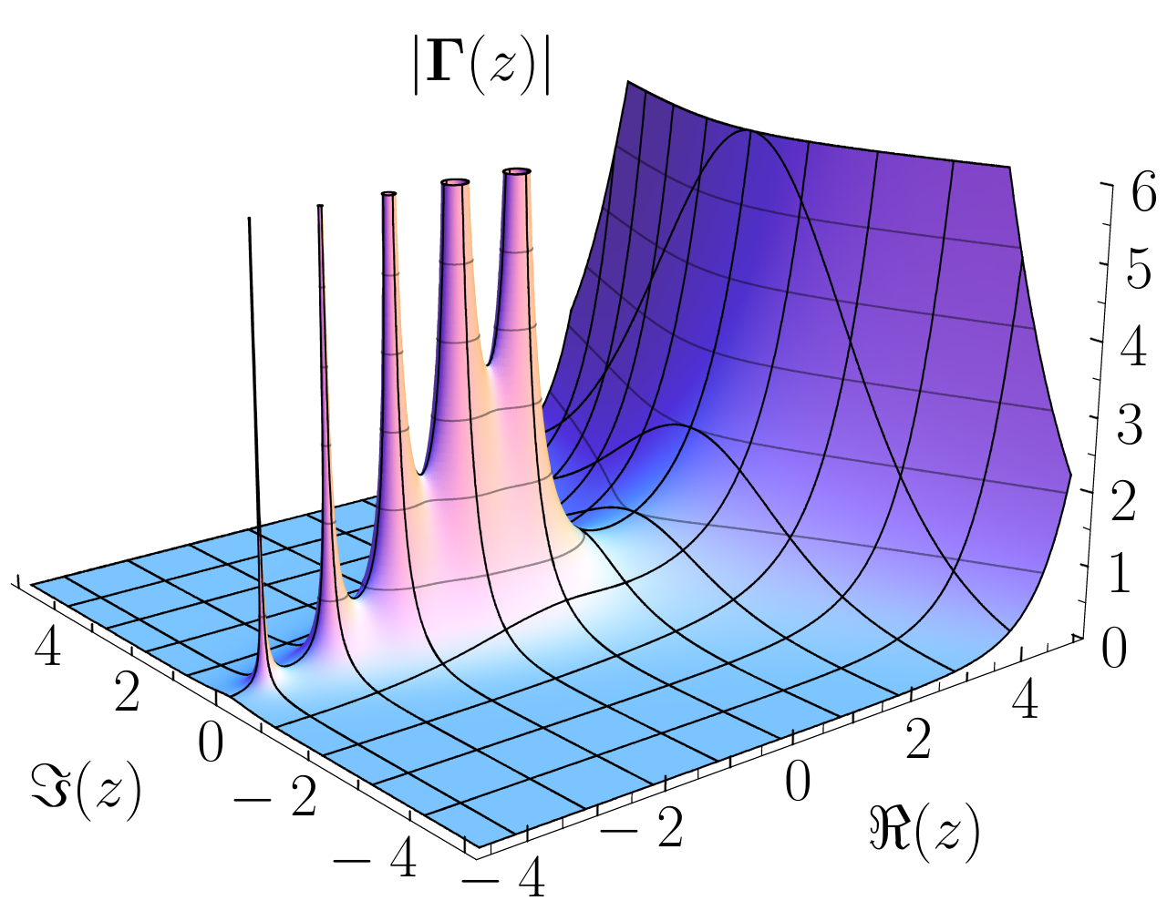
In complex analysis (a branch of mathematics), a pole is a certain type of singularity of a complex-valued function of a complex variable. It is the simplest type of non-removable singularity of such a function (see essential singularity). Technically, a point z0 is a pole of a function f if it is a zero of the function 1/f and 1/f is holomorphic (i.e. complex differentiable) in some neighbourhood of z0.

A function f is meromorphic in an open set U if for every point z of U there is a neighborhood of z in which at least one of f and 1/f is holomorphic.

If f is meromorphic in U, then a zero of f is a pole of 1/f, and a pole of f is a zero of 1/f. This induces a duality between zeros and poles, that is fundamental for the study of meromorphic functions. For example, if a function is meromorphic on the whole complex plane plus the point at infinity, then the sum of the multiplicities of its poles equals the sum of the multiplicities of its zeros.

Definitions

[edit]

A function of a complex variable z is holomorphic in an open domain U if it is differentiable with respect to z at every point of U. Equivalently, it is holomorphic if it is analytic, that is, if its Taylor series exists at every point of U, and converges to the function in some neighbourhood of the point. A function is meromorphic in U if every point of U has a neighbourhood such that at least one of f and 1/f is holomorphic in it.

A zero of a meromorphic function f is a complex number z such that f(z) = 0. A pole of f is a zero of 1/f.

If f is a function that is meromorphic in a neighbourhood of a point of the complex plane, then there exists an integer n such that

is holomorphic and nonzero in a neighbourhood of (this is a consequence of the analytic property). If n > 0, then is a pole of order (or multiplicity) n of f. If n < 0, then is a zero of order of f. Simple zero and simple pole are terms used for zeroes and poles of order Degree is sometimes used synonymously to order.

This characterization of zeros and poles implies that zeros and poles are isolated, that is, every zero or pole has a neighbourhood that does not contain any other zero and pole.

Because of the order of zeros and poles being defined as a non-negative number n and the symmetry between them, it is often useful to consider a pole of order n as a zero of order n and a zero of order n as a pole of order n. In this case a point that is neither a pole nor a zero is viewed as a pole (or zero) of order 0.

A meromorphic function may have infinitely many zeros and poles. This is the case for the gamma function (see the image in the infobox), which is meromorphic in the whole complex plane, and has a simple pole at every non-positive integer. The Riemann zeta function is also meromorphic in the whole complex plane, with a single pole of order 1 at z = 1. Its zeros in the left halfplane are all the negative even integers, and the Riemann hypothesis is the conjecture that all other zeros are along Re(z) = 1/2.

In a neighbourhood of a point a nonzero meromorphic function f is the sum of a Laurent series with at most finite principal part (the terms with negative index values):

where n is an integer, and Again, if n > 0 (the sum starts with , the principal part has n terms), one has a pole of order n, and if n ≤ 0 (the sum starts with , there is no principal part), one has a zero of order .

At infinity

[edit]

A function is meromorphic at infinity if it is meromorphic in some neighbourhood of infinity (that is outside some disk), and there is an integer n such that

exists and is a nonzero complex number.

In this case, the point at infinity is a pole of order n if n > 0, and a zero of order if n < 0.

For example, a polynomial of degree n has a pole of degree n at infinity.

The complex plane extended by a point at infinity is called the Riemann sphere.

If f is a function that is meromorphic on the whole Riemann sphere, then it has a finite number of zeros and poles, and the sum of the orders of its poles equals the sum of the orders of its zeros.

Every rational function is meromorphic on the whole Riemann sphere, and, in this case, the sum of orders of the zeros or of the poles is the maximum of the degrees of the numerator and the denominator.

Examples

[edit]
A polynomial of degree 9 has a pole of order 9 at ∞, here plotted by domain coloring of the Riemann sphere.
  • The function
is meromorphic on the whole Riemann sphere. It has a pole of order 1 or simple pole at and a simple zero at infinity.
  • The function
is meromorphic on the whole Riemann sphere. It has a pole of order 2 at and a pole of order 3 at . It has a simple zero at and a quadruple zero at infinity.
  • The function
is meromorphic in the whole complex plane, but not at infinity. It has poles of order 1 at . This can be seen from Euler's formula.
  • The function
has a single pole at infinity of order 1, and a single zero at the origin.

All above examples except for the third are rational functions. For a general discussion of zeros and poles of such functions, see Pole–zero plot § Continuous-time systems.

Function on a curve

[edit]

The concept of zeros and poles extends naturally to functions on a complex curve, that is complex analytic manifold of dimension one (over the complex numbers). The simplest examples of such curves are the complex plane and the Riemann surface. This extension is done by transferring structures and properties through charts, which are analytic isomorphisms.

More precisely, let f be a function from a complex curve M to the complex numbers. This function is holomorphic (resp. meromorphic) in a neighbourhood of a point z of M if there is a chart such that is holomorphic (resp. meromorphic) in a neighbourhood of Then, z is a pole or a zero of order n if the same is true for

If the curve is compact, and the function f is meromorphic on the whole curve, then the number of zeros and poles is finite, and the sum of the orders of the poles equals the sum of the orders of the zeros. This is one of the basic facts that are involved in Riemann–Roch theorem.

See also

[edit]

References

[edit]
[edit]
Revisions and contributorsEdit on WikipediaRead on Wikipedia
from Grokipedia
In complex analysis, zeros and poles are key features of holomorphic functions, where a zero is a point z0z_0 in the complex plane at which the function f(z)f(z) evaluates to zero, and a pole is an isolated singularity where f(z)f(z) tends to infinity. The order or multiplicity of a zero at z0z_0 is the smallest positive integer mm such that f(z)=(zz0)mg(z)f(z) = (z - z_0)^m g(z) for some holomorphic function gg with g(z0)0g(z_0) \neq 0, while a pole of order mm at z0z_0 occurs when 1/f(z)1/f(z) has a zero of order mm there, equivalently expressed as f(z)=(zz0)mh(z)f(z) = (z - z_0)^{-m} h(z) with holomorphic h(z0)0h(z_0) \neq 0. These concepts extend to meromorphic functions, which are holomorphic everywhere except at isolated poles, allowing the study of functions like the or the , the latter having simple poles at non-positive integers. Zeros and poles play a central role in residue theory, where the residue at a simple pole is given by limzz0(zz0)f(z)\lim_{z \to z_0} (z - z_0) f(z), facilitating the computation of contour integrals via the : Cf(z)dz=2πiRes(f,zk)\oint_C f(z) \, dz = 2\pi i \sum \operatorname{Res}(f, z_k) for poles inside a closed contour CC. A cornerstone result is the argument principle, which equates the winding number of f(C)f(C) around the origin to the difference between the number of zeros and poles (counted with multiplicity) inside CC: 12πiCf(z)f(z)dz=NP\frac{1}{2\pi i} \oint_C \frac{f'(z)}{f(z)} \, dz = N - P. This principle underpins applications in locating zeros (e.g., for bounding zero counts) and analyzing global behavior, such as the via zeta function zeros. Beyond , zeros and poles appear in control systems, where they determine stability through root locus plots, and in for filter design.

Core Concepts

Zeros of Analytic Functions

In , a zero of a ff defined on an ΩC\Omega \subset \mathbb{C} is a point z0Ωz_0 \in \Omega such that f(z0)=0f(z_0) = 0, provided that ff is not identically zero throughout any neighborhood of z0z_0. This definition ensures that the zero reflects a genuine vanishing of the function at that point without the function being trivially zero nearby. Holomorphic functions, being analytic everywhere in their domain, allow zeros to be characterized precisely through their local expansions. Near a zero z0z_0, the function ff admits a expansion f(z)=n=1an(zz0)nf(z) = \sum_{n=1}^\infty a_n (z - z_0)^n in some disk D(z0,r)ΩD(z_0, r) \subset \Omega, since the constant term vanishes. If the lowest-order non-zero is am0a_m \neq 0 with m1m \geq 1, then f(z)=(zz0)mg(z)f(z) = (z - z_0)^m g(z), where g(z)=k=0am+k(zz0)kg(z) = \sum_{k=0}^\infty a_{m+k} (z - z_0)^k is holomorphic in the same disk and g(z0)=am0g(z_0) = a_m \neq 0. This local factorization highlights the multiplicity mm of the zero, capturing how the function approaches zero like a power of the distance from z0z_0. Zeros of non-constant holomorphic functions are isolated, meaning there exists a punctured neighborhood around each zero containing no other zeros. If a sequence of distinct zeros accumulates at a point in the domain, then ff must be identically zero on the connected component containing that . This isolation property distinguishes zeros from cases where the function might be extended holomorphically after removal of singularities, as zeros occur at points where ff is already defined and holomorphic but vanishes. The concept of a "zero" traces its origins to the roots of polynomial equations and was extended by Augustin-Louis Cauchy to the vanishing points of analytic functions in his pioneering 19th-century development of complex function theory.

Poles of Analytic Functions

In complex analysis, a pole of an analytic function ff at a point z0z_0 is defined as an isolated singularity where limzz0f(z)=\lim_{z \to z_0} |f(z)| = \infty. This means there exists a deleted neighborhood around z0z_0 in which ff is holomorphic and nonzero, ensuring the singularity is isolated and the function tends to infinity in magnitude as zz approaches z0z_0. Near a pole z0z_0 of order n1n \geq 1, the function ff admits a local representation of the form f(z)=(zz0)nh(z),f(z) = (z - z_0)^{-n} h(z), where hh is holomorphic in a neighborhood of z0z_0 and h(z0)0h(z_0) \neq 0. This expression captures the singular behavior, with the negative power (zz0)n(z - z_0)^{-n} dominating as zz approaches z0z_0, while h(z)h(z) remains finite and nonzero at that point. Poles are classified as non-essential isolated singularities, in contrast to essential singularities where the behavior is more erratic. In the Laurent series expansion of ff around z0z_0, f(z)=k=ak(zz0)kf(z) = \sum_{k=-\infty}^{\infty} a_k (z - z_0)^k, a pole is characterized by the principal part (the sum of terms with negative powers) having only finitely many nonzero coefficients, specifically up to the term (zz0)n(z - z_0)^{-n} where an0a_{-n} \neq 0 and ak=0a_k = 0 for all k<nk < -n. The poles of ff are closely related to the zeros of its reciprocal 1/f1/f, in that if z0z_0 is a pole of ff of order nn, then z0z_0 is a zero of 1/f1/f of the same order nn.

Orders and Multiplicities

The order of a zero of an analytic function ff at a point z0z_0, where f(z0)=0f(z_0) = 0, is defined as the smallest positive integer mm such that the mm-th derivative f(m)(z0)0f^{(m)}(z_0) \neq 0. Equivalently, in the Taylor series expansion of ff around z0z_0, given by k=0ak(zz0)k\sum_{k=0}^{\infty} a_k (z - z_0)^k, the multiplicity mm is the smallest integer kk for which the coefficient ak0a_k \neq 0. This multiplicity quantifies how "repeated" the zero is, reflecting the local behavior near z0z_0 where f(z)f(z) vanishes to order mm. For poles, the order at an isolated singularity z0z_0 is the smallest positive integer nn such that (zz0)nf(z)(z - z_0)^n f(z) is analytic at z0z_0 and (zz0)nf(z0)0(z - z_0)^n f(z_0) \neq 0. In the Laurent series k=ak(zz0)k\sum_{k=-\infty}^{\infty} a_k (z - z_0)^k, the multiplicity nn corresponds to the most negative power with a nonzero coefficient, i.e., n=min{kak0,k<0}n = -\min\{k \mid a_k \neq 0, k < 0\}. This order indicates the severity of the singularity, with f(z)f(z) approaching infinity as (zz0)n(z - z_0)^{-n} near z0z_0. To compute the order of a zero, one can evaluate successive derivatives: if f(z0)=f(z0)==f(m1)(z0)=0f(z_0) = f'(z_0) = \cdots = f^{(m-1)}(z_0) = 0 but f(m)(z0)0f^{(m)}(z_0) \neq 0, then the multiplicity is mm. Alternatively, the limit limzz0(zz0)mf(z)=c0,\lim_{z \to z_0} (z - z_0)^{-m} f(z) = c \neq 0, \infty confirms multiplicity mm. For poles, a similar limit test applies: limzz0(zz0)nf(z)=d0,\lim_{z \to z_0} (z - z_0)^{n} f(z) = d \neq 0, \infty verifies order nn, while lower powers yield infinity and higher powers yield zero. Zeros and poles of order 1 are termed simple, whereas higher orders are multiple. A simple zero satisfies f(z0)=0f(z_0) = 0 and f(z0)0f'(z_0) \neq 0, while a simple pole has limzz0(zz0)f(z)0,\lim_{z \to z_0} (z - z_0) f(z) \neq 0, \infty. Multiple zeros or poles, with order greater than 1, exhibit more pronounced local flattening or blow-up, respectively, as captured by the series expansions.

Extension to the Riemann Sphere

Zeros and Poles at Infinity

To analyze the behavior of an analytic function f(z)f(z) at the point at infinity, consider the coordinate inversion z=1/wz = 1/w, which maps the neighborhood of infinity to the neighborhood of w=0w = 0. Define g(w)=f(1/w)g(w) = f(1/w); then, z=z = \infty is a zero of ff if and only if w=0w = 0 is a zero of gg, and z=z = \infty is a pole of ff if and only if w=0w = 0 is a pole of gg. The order of a zero or pole of ff at infinity equals the order of the corresponding zero or pole of gg at w=0w = 0. For instance, if g(w)g(w) admits a Taylor expansion g(w)=amwm+am+1wm+1+g(w) = a_m w^m + a_{m+1} w^{m+1} + \cdots with am0a_m \neq 0 and m1m \geq 1, then ff has a zero of order mm at \infty. Similarly, if the Laurent series of gg at w=0w = 0 has principal part bmwm++b1w1b_{-m} w^{-m} + \cdots + b_{-1} w^{-1} with bm0b_{-m} \neq 0 and m1m \geq 1, then ff has a pole of order mm at \infty. This classification aligns with asymptotic behavior as z|z| \to \infty: ff has a zero at \infty if limzf(z)=0\lim_{|z| \to \infty} |f(z)| = 0, and a pole at \infty if limzf(z)=\lim_{|z| \to \infty} |f(z)| = \infty (or equivalently, limz1/f(z)=0\lim_{|z| \to \infty} |1/f(z)| = 0). For example, the function f(z)=1/zf(z) = 1/z satisfies g(w)=wg(w) = w, which has a simple zero at w=0w = 0, so ff has a simple zero at \infty; asymptotically, f(z)0|f(z)| \to 0 as z|z| \to \infty. Conversely, f(z)=zf(z) = z gives g(w)=1/wg(w) = 1/w, a simple pole at w=0w = 0, so ff has a simple pole at \infty, with f(z)|f(z)| \to \infty as z|z| \to \infty. More generally, a polynomial of degree nn has a pole of order nn at \infty, while a rational function where the degree of the denominator exceeds that of the numerator by kk has a zero of order kk at \infty.

Compactification and the Extended Plane

The Riemann sphere, denoted C^\hat{\mathbb{C}}, is the extended complex plane formed by adjoining a point at infinity to the complex plane C\mathbb{C}, yielding C^=C{}\hat{\mathbb{C}} = \mathbb{C} \cup \{\infty\}. This construction compactifies the plane, transforming it into a topologically closed surface homeomorphic to the two-dimensional sphere S2S^2 through stereographic projection from the north pole. The stereographic projection provides a bijective correspondence between points in C\mathbb{C} and points on S2S^2 excluding the north pole, with the north pole representing infinity, enabling a uniform geometric interpretation of complex analysis on a compact manifold. The Riemann sphere, named after Bernhard Riemann for his foundational contributions to complex analysis, was developed to compactify the complex plane, allowing for a consistent treatment of singularities, including those at infinity, within the framework of Riemann surfaces. This topological embedding facilitates the analysis of meromorphic functions by embedding the plane into a compact space where global properties, such as the balance of singularities, can be studied holomorphically. On the Riemann sphere C^\hat{\mathbb{C}}, every non-constant meromorphic function defined on C\mathbb{C} extends to a meromorphic function with an equal number of zeros and poles, counted with multiplicity, reflecting the compact nature of the surface and the degree of the corresponding holomorphic map to C^\hat{\mathbb{C}}. Holomorphic maps from C^\hat{\mathbb{C}} to itself are precisely the rational functions, which arise naturally as the field of meromorphic functions on this surface. Under the inversion transformation z1/zz \mapsto 1/z, which is a biholomorphic automorphism of C^\hat{\mathbb{C}}, poles at infinity transform into zeros at the origin, underscoring the symmetry in treating finite and infinite singularities uniformly.

Illustrative Examples

In Rational Functions

A rational function in the complex plane is expressed as f(z)=p(z)q(z)f(z) = \frac{p(z)}{q(z)}, where p(z)p(z) and q(z)q(z) are polynomials with complex coefficients, assumed to be in reduced form with no common roots. The zeros of f(z)f(z) occur at the roots of the numerator polynomial p(z)p(z), provided the denominator q(z)q(z) does not vanish there, while the poles arise at the roots of the denominator q(z)q(z), assuming the numerator does not vanish at those points. The multiplicity, or order, of a zero or pole in a rational function inherits directly from the multiplicity of the corresponding root in the numerator or denominator polynomial. For instance, consider f(z)=(z1)2z+1f(z) = \frac{(z-1)^2}{z+1}; here, p(z)=(z1)2p(z) = (z-1)^2 has a root of multiplicity 2 at z=1z=1, yielding a zero of order 2 for f(z)f(z) at that point, while q(z)=z+1q(z) = z+1 has a simple root at z=1z=-1, resulting in a pole of order 1. The behavior of a rational function at infinity is determined by comparing the degrees of the numerator and denominator polynomials, say degp=m\deg p = m and degq=n\deg q = n. If m<nm < n, then f(z)f(z) has a zero at infinity of order nmn - m; if m>nm > n, it has a pole at infinity of order mnm - n; and if m=nm = n, the function approaches a finite non-zero limit at infinity. Partial fraction decomposition provides an explicit way to express a as a sum of terms that isolate the principal parts near each pole, facilitating analysis of singularities. For example, the decomposition of 1z21=1(z1)(z+1)\frac{1}{z^2 - 1} = \frac{1}{(z-1)(z+1)} is 1/2z11/2z+1\frac{1/2}{z-1} - \frac{1/2}{z+1}, where the residues 1/21/2 and 1/2-1/2 are computed at the simple poles z=1z=1 and z=1z=-1, respectively.

In Entire and Meromorphic Functions

Entire functions are holomorphic everywhere in the finite and thus possess no poles there, though they may exhibit an at infinity. A prototypical example is the sine function sinz\sin z, which has simple zeros at all multiples of π\pi, namely z=nπz = n\pi for nZn \in \mathbb{Z}, forming an infinite set along the real axis. These zeros are isolated, and sinz\sin z can be expressed via the as an incorporating these points, highlighting how transcendental entire functions accommodate countably many zeros without singularities in the plane. Meromorphic functions, by contrast, are holomorphic except at isolated poles and provide examples where both zeros and poles occur infinitely often. The tanz\tan z, for instance, is meromorphic on the with simple poles at z=(n+1/2)πz = (n + 1/2)\pi for all integers nn, located along axis at odd multiples of π/2\pi/2. Similarly, the Γ(z)\Gamma(z) is meromorphic with simple poles precisely at the non-positive integers z=0,1,2,z = 0, -1, -2, \dots, and no zeros anywhere in the plane. These poles arise from the and reflection formula of Γ(z)\Gamma(z), underscoring the discrete yet infinite nature of singularities in such functions. In transcendental settings, zeros and poles remain isolated within the domain of holomorphy but can accumulate only at essential singularities or at infinity. For example, the function 1/sin(1/z)1/\sin(1/z) is meromorphic on C{0}\mathbb{C} \setminus \{0\} with simple poles at z=1/(nπ)z = 1/(n\pi) for nonzero integers nn, accumulating at the origin, where sin(1/z)\sin(1/z) itself has an essential singularity. This accumulation is permitted because the point of accumulation lies outside the domain, consistent with the isolation principle for meromorphic functions; by the identity theorem, no such clustering can occur interior to the region without implying the function is identically zero or non-meromorphic. Picard's little theorem extends this perspective, stating that a non-constant on the omits at most two values in the extended , which implies that it attains all but possibly two complex values infinitely often—consequently featuring infinitely many zeros and poles in the plane, counted with multiplicity. This result, derived from the behavior near essential singularities via the Casorati-Weierstrass theorem, emphasizes the richness of transcendental meromorphic functions compared to their rational counterparts.

Theoretical Implications

The Argument Principle

The argument principle, also known as Cauchy's argument principle, is a fundamental theorem in complex analysis that relates the number of zeros and poles of a meromorphic function inside a closed contour to an integral involving the function along that contour. Specifically, for a meromorphic function ff in a domain containing a simple closed positively oriented contour γ\gamma and its interior, with no zeros or poles on γ\gamma, the integral 12πiγdff=NP\frac{1}{2\pi i} \int_\gamma \frac{df}{f} = N - P, where NN is the number of zeros inside γ\gamma (counted with multiplicity) and PP is the number of poles inside γ\gamma (also counted with multiplicity). This equality holds because the integrand ff\frac{f'}{f} has simple poles at the zeros and poles of ff, with residues equal to the respective multiplicities. The derivation follows directly from the residue theorem applied to the meromorphic differential form dff\frac{df}{f}. At a zero of order mm, the Laurent series of ff yields a residue of mm for ff\frac{f'}{f}, while at a pole of order mm, the residue is m-m. Summing these residues over all singularities inside γ\gamma and applying the residue theorem gives the net count NPN - P. Equivalently, the principle can be expressed in terms of the change in argument: Δargf(γ)=2π(NP)\Delta \arg f(\gamma) = 2\pi (N - P), since the integral 12πiγdff\frac{1}{2\pi i} \int_\gamma \frac{df}{f} equals 12πΔargf(γ)\frac{1}{2\pi} \Delta \arg f(\gamma). Geometrically, this result interprets NPN - P as the winding number of the image curve f(γ)f(\gamma) around the origin in the complex plane. The curve f(γ)f(\gamma) encircles 0 exactly NPN - P times (with positive orientation), reflecting how the zeros contribute positively and poles negatively to the total encirclements. This winding number perspective underscores the principle's role in counting singularities without explicit location. Rouché's theorem extends the argument principle by enabling comparisons of zero and pole counts inside contours through dominant functions on the boundary. If g(z)<f(z)|g(z)| < |f(z)| on γ\gamma for holomorphic ff and gg with no zeros or poles on γ\gamma, then ff and f+gf + g have the same number of zeros inside γ\gamma, as their images wind around 0 the same number of times. This allows locating zeros and poles by perturbing known functions whose singularity counts are straightforward.

Zeros, Poles, and Integration on Curves

In , the residue of a f(z)f(z) at a simple pole z0z_0 is defined as Res(f,z0)=limzz0(zz0)f(z)\operatorname{Res}(f, z_0) = \lim_{z \to z_0} (z - z_0) f(z), which extracts the of the (zz0)1(z - z_0)^{-1} term in the expansion of ff around z0z_0. This residue quantifies the singularity's contribution to contour integrals enclosing z0z_0, as per the , where γf(z)dz=2πiRes(f,zk)\int_\gamma f(z) \, dz = 2\pi i \sum \operatorname{Res}(f, z_k) for poles zkz_k inside the closed curve γ\gamma. At a zero of ff, where ff is analytic, the contains only non-negative powers, so the residue is zero, meaning zeros do not contribute to such integrals. An extension of applies this to locate zeros and poles via : for a meromorphic ff with no zeros or poles on the simple closed curve γ\gamma, the integral 12πiγf(z)f(z)dz=NP\frac{1}{2\pi i} \int_\gamma \frac{f'(z)}{f(z)} \, dz = N - P, where NN counts the zeros inside γ\gamma (with multiplicity) and PP counts the poles (with order). This formula arises from the ff\frac{f'}{f}, whose residues at zeros and poles are +1+1 and 1-1 times their multiplicities or orders, respectively, enabling the net count without solving f(z)=0f(z) = 0 explicitly. In practice, this facilitates numerical root-finding for complex functions by evaluating γffdz\int_\gamma \frac{f'}{f} \, dz over trial contours, such as rectangles or circles, to determine NN and iteratively refine regions containing zeros; for instance, adaptive subdivision of the uses the approximation of the to isolate roots efficiently. Such methods avoid direct factoring or iterative solvers like Newton-Raphson, particularly for high-degree polynomials or transcendental functions where explicit zeros are intractable. The global residue theorem extends this balance to the entire C^\hat{\mathbb{C}}: for a on C^\hat{\mathbb{C}}, the sum of all residues, including the residue at (defined as Res(f,)=12πiγ=Rf(z)dz-\operatorname{Res}(f, \infty) = \frac{1}{2\pi i} \int_{|\gamma|=R} f(z) \, dz for large RR), equals zero, reflecting the topological closure where zeros and poles must equilibrate globally. This ensures that the total "defect" from singularities, weighted by residues, vanishes over the compactified plane.

References

Add your contribution
Related Hubs
User Avatar
No comments yet.