Stability theory

This section does not cite any sources. Please help improve this section by adding citations to reliable sources. Unsourced material may be challenged and removed. (December 2024) (Learn how and when to remove this message)

Many parts of the qualitative theory of differential equations and dynamical systems deal with asymptotic properties of solutions and the trajectories—what happens with the system after a long period of time. The simplest kind of behavior is exhibited by equilibrium points, or fixed points, and by periodic orbits. If a particular orbit is well understood, it is natural to ask next whether a small change in the initial condition will lead to similar behavior. Stability theory addresses the following questions: Will a nearby orbit indefinitely stay close to a given orbit? Will it converge to the given orbit? In the former case, the orbit is called stable; in the latter case, it is called asymptotically stable and the given orbit is said to be attracting.

An equilibrium solution ${\displaystyle f_{e}}$ to an autonomous system of first order ordinary differential equations is called:

• stable if for every (small) ${\displaystyle \epsilon >0}$, there exists a ${\displaystyle \delta >0}$ such that every solution ${\displaystyle f(t)}$ having initial conditions within distance ${\displaystyle \delta }$ i.e. ${\displaystyle \|f(t_{0})-f_{e}\|<\delta }$ of the equilibrium remains within distance ${\displaystyle \epsilon }$ i.e. ${\displaystyle \|f(t)-f_{e}\|<\epsilon }$ for all ${\displaystyle t\geq t_{0}}$.
• asymptotically stable if it is stable and, in addition, there exists ${\displaystyle \delta _{0}>0}$ such that whenever ${\displaystyle \|f(t_{0})-f_{e}\|<\delta _{0}}$ then ${\displaystyle f(t)\rightarrow f_{e}}$as ${\displaystyle t\rightarrow \infty }$.

Stability means that the trajectories do not change too much under small perturbations. The opposite situation, where a nearby orbit is getting repelled from the given orbit, is also of interest. In general, perturbing the initial state in some directions results in the trajectory asymptotically approaching the given one and in other directions to the trajectory getting away from it. There may also be directions for which the behavior of the perturbed orbit is more complicated (neither converging nor escaping completely), and then stability theory does not give sufficient information about the dynamics.

One of the key ideas in stability theory is that the qualitative behavior of an orbit under perturbations can be analyzed using the linearization of the system near the orbit. In particular, at each equilibrium of a smooth dynamical system with an n-dimensional phase space, there is a certain n×n matrix A whose eigenvalues characterize the behavior of the nearby points (Hartman–Grobman theorem). More precisely, if all eigenvalues are negative real numbers or complex numbers with negative real parts then the point is a stable attracting fixed point, and the nearby points converge to it at an exponential rate, cf Lyapunov stability and exponential stability. If none of the eigenvalues are purely imaginary (or zero) then the attracting and repelling directions are related to the eigenspaces of the matrix A with eigenvalues whose real part is negative and, respectively, positive. Analogous statements are known for perturbations of more complicated orbits.

This section does not cite any sources. Please help improve this section by adding citations to reliable sources. Unsourced material may be challenged and removed. (December 2024) (Learn how and when to remove this message)

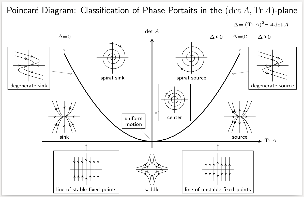
The paradigmatic case is the stability of the origin under the linear autonomous differential equation ${\displaystyle {\dot {X}}=AX}$ where ${\displaystyle X={\begin{bmatrix}x\\y\end{bmatrix}}}$ and ${\displaystyle A}$ is a 2×2 matrix.

We would sometimes perform change-of-basis by ${\displaystyle X'=CX}$ for some invertible matrix ${\displaystyle C}$, which gives ${\displaystyle {\dot {X}}'=C^{-1}ACX'}$. We say ${\displaystyle C^{-1}AC}$ is "${\displaystyle A}$ in the new basis". Since ${\displaystyle \det A=\det C^{-1}AC}$ and ${\displaystyle \operatorname {tr} A=\operatorname {tr} C^{-1}AC}$, we can classify the stability of origin using ${\displaystyle \det A}$ and ${\displaystyle \operatorname {tr} A}$, while freely using change-of-basis.

If ${\displaystyle \det A=0}$, then the rank of ${\displaystyle A}$ is zero or one.

• If the rank is zero, then ${\displaystyle A=0}$, and there is no flow.
• If the rank is one, then ${\displaystyle \ker A}$ and ${\displaystyle \operatorname {im} A}$ are both one-dimensional.
  • If ${\displaystyle \ker A=\operatorname {im} A}$, then let ${\displaystyle v}$ span ${\displaystyle \ker A}$, and let ${\displaystyle w}$ be a preimage of ${\displaystyle v}$, then in ${\displaystyle \{v,w\}}$ basis, ${\displaystyle A={\begin{bmatrix}0&1\\0&0\end{bmatrix}}}$, and so the flow is a shearing along the ${\displaystyle v}$ direction. In this case, ${\displaystyle \operatorname {tr} A=0}$.
  • If ${\displaystyle \ker A\neq \operatorname {im} A}$, then let ${\displaystyle v}$ span ${\displaystyle \ker A}$ and let ${\displaystyle w}$ span ${\displaystyle \operatorname {im} A}$, then in ${\displaystyle \{v,w\}}$ basis, ${\displaystyle A={\begin{bmatrix}0&0\\0&a\end{bmatrix}}}$ for some nonzero real number ${\displaystyle a}$.
    • If ${\displaystyle \operatorname {tr} A>0}$, then it is unstable, diverging at a rate of ${\displaystyle a}$ from ${\displaystyle \ker A}$ along parallel translates of ${\displaystyle \operatorname {im} A}$.
    • If ${\displaystyle \operatorname {tr} A<0}$, then it is stable, converging at a rate of ${\displaystyle a}$ to ${\displaystyle \ker A}$ along parallel translates of ${\displaystyle \operatorname {im} A}$.

If ${\displaystyle \det A\neq 0}$, we first find the Jordan normal form of the matrix, to obtain a basis ${\displaystyle \{v,w\}}$ in which ${\displaystyle A}$ is one of three possible forms:

• ${\displaystyle {\begin{bmatrix}a&0\\0&b\end{bmatrix}}}$ where ${\displaystyle a,b\neq 0}$.
  • If ${\displaystyle a,b>0}$, then ${\displaystyle {\begin{cases}4\det A-(\operatorname {tr} A)^{2}=-(a-b)^{2}\leq 0\\\det A=ab>0\end{cases}}}$. The origin is a source, with integral curves of form ${\displaystyle y=cx^{b/a}}$
  • Similarly for ${\displaystyle a,b<0}$. The origin is a sink.
  • If ${\displaystyle a>0>b}$ or ${\displaystyle a<0<b}$, then ${\displaystyle \det A<0}$, and the origin is a saddle point. with integral curves of form ${\displaystyle y=cx^{-|b/a|}}$.
• ${\displaystyle {\begin{bmatrix}a&1\\0&a\end{bmatrix}}}$ where ${\displaystyle a\neq 0}$. This can be further simplified by a change-of-basis with ${\displaystyle C={\begin{bmatrix}1/a&0\\0&1\end{bmatrix}}}$, after which ${\displaystyle A=a{\begin{bmatrix}1&1\\0&1\end{bmatrix}}}$. We can explicitly solve for ${\displaystyle {\dot {X}}=AX}$ with ${\displaystyle A=a{\begin{bmatrix}1&1\\0&1\end{bmatrix}}}$. The solution is ${\displaystyle X(t)=e^{At}X(0)}$ with ${\displaystyle e^{At}=e^{at}{\begin{bmatrix}1&at\\0&1\end{bmatrix}}}$. This case is called the "degenerate node". The integral curves in this basis are central dilations of ${\displaystyle x=y\ln y}$, plus the x-axis.
  • If ${\displaystyle \operatorname {tr} A>0}$, then the origin is an degenerate source. Otherwise it is a degenerate sink.
  • In both cases, ${\displaystyle 4\det A-(\operatorname {tr} A)^{2}=0}$
• ${\displaystyle a{\begin{bmatrix}\cos \theta &\sin \theta \\-\sin \theta &\cos \theta \end{bmatrix}}}$ where ${\displaystyle a>0,\theta \in (-\pi ,\pi ]}$. In this case, ${\displaystyle 4\det A-(\operatorname {tr} A)^{2}=(2a\sin \theta )^{2}\geq 0}$.
  • If ${\displaystyle \theta \in (-\pi ,-\pi /2)\cup (\pi /2,\pi ]}$, then this is a spiral sink. In this case, ${\displaystyle {\begin{cases}4\det A-(\operatorname {tr} A)^{2}>0\\\operatorname {tr} A<0\end{cases}}}$. The integral lines are logarithmic spirals.
  • If ${\displaystyle \theta \in (-\pi /2,\pi /2)}$, then this is a spiral source. In this case, ${\displaystyle {\begin{cases}4\det A-(\operatorname {tr} A)^{2}>0\\\operatorname {tr} A>0\end{cases}}}$. The integral lines are logarithmic spirals.
  • If ${\displaystyle \theta =-\pi /2,\pi /2}$, then this is a rotation ("neutral stability") at a rate of ${\displaystyle a}$, moving neither towards nor away from origin. In this case, ${\displaystyle \operatorname {tr} A=0}$. The integral lines are circles.

The summary is shown in the stability diagram on the right. In each case, except the case of ${\displaystyle 4\det A-(\operatorname {tr} A)^{2}=0}$, the values ${\displaystyle (\operatorname {tr} A,\det A)}$ allows unique classification of the type of flow.

For the special case of ${\displaystyle 4\det A-(\operatorname {tr} A)^{2}=0}$, there are two cases that cannot be distinguished by ${\displaystyle (\operatorname {tr} A,\det A)}$. In both cases, ${\displaystyle A}$ has only one eigenvalue, with algebraic multiplicity 2.

• If the eigenvalue has a two-dimensional eigenspace (geometric multiplicity 2), then the system is a central node (sometimes called a "star", or "dicritical node") which is either a source (when ${\displaystyle \operatorname {tr} A>0}$) or a sink (when ${\displaystyle \operatorname {tr} A<0}$).^[2]
• If it has a one-dimensional eigenspace (geometric multiplicity 1), then the system is a degenerate node (if ${\displaystyle \det A>0}$) or a shearing flow (if ${\displaystyle \det A=0}$).

When ${\displaystyle \operatorname {tr} A=0}$, we have ${\displaystyle \det e^{At}=e^{\operatorname {tr} (A)t}=1}$, so the flow is area-preserving. In this case, the type of flow is classified by ${\displaystyle \det A}$.

• If ${\displaystyle \det A>0}$, then it is a rotation ("neutral stability") around the origin.
• If ${\displaystyle \det A=0}$, then it is a shearing flow.
• If ${\displaystyle \det A<0}$, then the origin is a saddle point.

This section does not cite any sources. Please help improve this section by adding citations to reliable sources. Unsourced material may be challenged and removed. (December 2024) (Learn how and when to remove this message)

The simplest kind of an orbit is a fixed point, or an equilibrium. If a mechanical system is in a stable equilibrium state then a small push will result in a localized motion, for example, small oscillations as in the case of a pendulum. In a system with damping, a stable equilibrium state is moreover asymptotically stable. On the other hand, for an unstable equilibrium, such as a ball resting on a top of a hill, certain small pushes will result in a motion with a large amplitude that may or may not converge to the original state.

There are useful tests of stability for the case of a linear system. Stability of a nonlinear system can often be inferred from the stability of its linearization.

Let f: R → R be a continuously differentiable function with a fixed point a, f(a) = a. Consider the dynamical system obtained by iterating the function f:

$${\displaystyle x_{n+1}=f(x_{n}),\quad n=0,1,2,\ldots .}$$

The fixed point a is stable if the absolute value of the derivative of f at a is strictly less than 1, and unstable if it is strictly greater than 1. This is because near the point a, the function f has a linear approximation with slope f'(a):

$${\displaystyle f(x)\approx f(a)+f'(a)\left(x-a\right).}$$

Thus

$${\displaystyle {\begin{aligned}x_{n+1}=f(x_{n})&\approx f(a)+f'(a)\left(x_{n}-a\right)\\&=a+f'(a)\left(x_{n}-a\right)\end{aligned}}}$$ $${\displaystyle \Rightarrow f'(a)\approx {\frac {x_{n+1}-a}{x_{n}-a}}}$$

which means that the derivative measures the rate at which the successive iterates approach the fixed point a or diverge from it. If the derivative at a is exactly 1 or −1, then more information is needed in order to decide stability.

There is an analogous criterion for a continuously differentiable map f: Rⁿ → Rⁿ with a fixed point a, expressed in terms of its Jacobian matrix at a, J_a(f). If all eigenvalues of J are real or complex numbers with absolute value strictly less than 1 then a is a stable fixed point; if at least one of them has absolute value strictly greater than 1 then a is unstable. Just as for n=1, the case of the largest absolute value being 1 needs to be investigated further — the Jacobian matrix test is inconclusive. The same criterion holds more generally for diffeomorphisms of a smooth manifold.

The stability of fixed points of a system of constant coefficient linear differential equations of first order can be analyzed using the eigenvalues of the corresponding matrix.

An autonomous system

$${\displaystyle x'=Ax,}$$

where x(t) ∈ Rⁿ and A is an n×n matrix with real entries, has a constant solution

$${\displaystyle x(t)=0.}$$

(In a different language, the origin 0 ∈ Rⁿ is an equilibrium point of the corresponding dynamical system.) This solution is asymptotically stable as t → ∞ ("in the future") if and only if for all eigenvalues λ of A, Re(λ) < 0. Similarly, it is asymptotically stable as t → −∞ ("in the past") if and only if for all eigenvalues λ of A, Re(λ) > 0. If there exists an eigenvalue λ of A with Re(λ) > 0 then the solution is unstable for t → ∞.

The stability of a linear system can be determined by solving the differential equation to find the eigenvalues, or without solving the equation by using the Routh–Hurwitz stability criterion. The eigenvalues of a matrix are the roots of its characteristic polynomial. A polynomial in one variable with real coefficients is called a Hurwitz polynomial if the real parts of all roots are strictly negative. The Routh–Hurwitz theorem implies a characterization of Hurwitz polynomials by means of an algorithm that avoids computing the roots.

Asymptotic stability of fixed points of a non-linear system can often be established using the Hartman–Grobman theorem.

Suppose that v is a C¹-vector field in Rⁿ which vanishes at a point p, v(p) = 0. Then the corresponding autonomous system

$${\displaystyle x'=v(x)}$$

has a constant solution

$${\displaystyle x(t)=p.}$$

Let J_p(v) be the n×n Jacobian matrix of the vector field v at the point p. If all eigenvalues of J have strictly negative real part then the solution is asymptotically stable. This condition can be tested using the Routh–Hurwitz criterion.

This section does not cite any sources. Please help improve this section by adding citations to reliable sources. Unsourced material may be challenged and removed. (December 2024) (Learn how and when to remove this message)

A general way to establish Lyapunov stability or asymptotic stability of a dynamical system is by means of Lyapunov functions.

• Chaos theory – Field of mathematics and science based on non-linear systems and initial conditions
• Ship stability – Ship response to disturbance from an upright condition
• Lyapunov stability – Property of a dynamical system where solutions near an equilibrium point remain so
• Hyperstability
• Linear stability – State of linear equations
• Orbital stability – Solution to a partial differential equation which remains close to the initial data
• Stability criterion
• Stability radius – Concept in mathematics
• Structural stability – Concept in mathematics
• von Neumann stability analysis – Numerical analysis procedure