Hubbry Logo
Fluorescence spectroscopyFluorescence spectroscopyMain
Open search
Fluorescence spectroscopy
Community hub
Fluorescence spectroscopy
logo
8 pages, 0 posts
0 subscribers
Be the first to start a discussion here.
Fluorescence spectroscopy
from Wikipedia
Atomic fluorescence spectroscopy analyzer for determination of mercury

Fluorescence spectroscopy (also known as fluorimetry or spectrofluorometry) is a type of electromagnetic spectroscopy that analyzes fluorescence from a sample. It involves using a beam of light, usually ultraviolet light, that excites the electrons in molecules of certain compounds and causes them to emit light; typically, but not necessarily, visible light. A complementary technique is absorption spectroscopy. In the special case of single molecule fluorescence spectroscopy, intensity fluctuations from the emitted light are measured from either single fluorophores, or pairs of fluorophores.

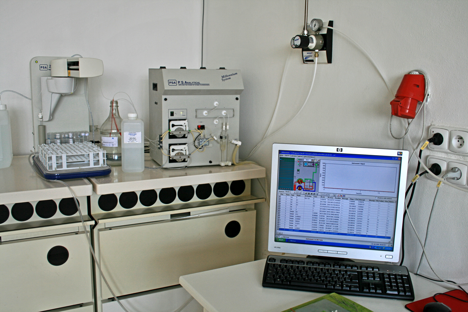
Devices that measure fluorescence are called fluorometers.

Theory

[edit]

Molecules have various states referred to as energy levels. Fluorescence spectroscopy is primarily concerned with electronic and vibrational states. Generally, the species being examined has a ground electronic state (a low energy state) of interest, and an excited electronic state of higher energy. Within each of these electronic states there are various vibrational states.[1]

In fluorescence, the species is first excited, by absorbing a photon, from its ground electronic state to one of the various vibrational states in the excited electronic state. Collisions with other molecules cause the excited molecule to lose vibrational energy until it reaches the lowest vibrational state of the excited electronic state. This process is often visualized with a Jablonski diagram.[1]

The molecule then drops down to one of the various vibrational levels of the ground electronic state again, emitting a photon in the process.[1] As molecules may drop down into any of several vibrational levels in the ground state, the emitted photons will have different energies, and thus frequencies. Therefore, by analysing the different frequencies of light emitted in fluorescent spectroscopy, along with their relative intensities, the structure of the different vibrational levels can be determined.

For atomic species, the process is similar; however, since atomic species do not have vibrational energy levels, the emitted photons are often at the same wavelength as the incident radiation. This process of re-emitting the absorbed photon is "resonance fluorescence" and while it is characteristic of atomic fluorescence, is seen in molecular fluorescence as well.[2]

In a typical fluorescence (emission) measurement, the excitation wavelength (the wavelength of the incident light used to excite the fluorophore) is fixed and the detection wavelength varies (producing an emission spectrum, while in a fluorescence excitation measurement the detection wavelength is fixed and the excitation wavelength is varied across a region of interest to produce an excitation spectrum. An excitation-emission matrix is obtained by recording the emission spectra resulting from a range of excitation wavelengths and combining them all together.[3][4] This is a three dimensional surface data set: emission intensity as a function of excitation and emission wavelengths, and is typically depicted as a contour map.

Instrumentation

[edit]

Two general types of instruments exist: filter fluorometers that use filters to isolate the incident light and fluorescent light and spectrofluorometers that use diffraction grating monochromators to isolate the incident light and fluorescent light.

Both types use the following scheme: the light from an excitation source passes through a filter or monochromator, and strikes the sample. A proportion of the incident light is absorbed by the sample, and some of the molecules in the sample fluoresce. The fluorescent light is emitted in all directions. Some of this fluorescent light passes through a second filter or monochromator and reaches a detector, which is usually placed at 90° to the incident light beam to minimize the risk of transmitted or reflected incident light reaching the detector.

A simplistic design of the components of a fluorimeter

Various light sources may be used as excitation sources, including lasers, LED, and lamps; xenon arcs and mercury-vapor lamps in particular. A laser only emits light of high irradiance at a very narrow wavelength interval, typically under 0.01 nm, which makes an excitation monochromator or filter unnecessary. The disadvantage of this method is that the wavelength of a laser cannot be changed by much. A mercury vapor lamp is a line lamp, meaning it emits light near peak wavelengths. By contrast, a xenon arc has a continuous emission spectrum with nearly constant intensity in the range from 300-800 nm and a sufficient irradiance for measurements down to just above 200 nm.

Filters and/or monochromators may be used in fluorimeters. A monochromator transmits light of an adjustable wavelength with an adjustable tolerance. The most common type of monochromator utilizes a diffraction grating, that is, collimated light illuminates a grating and exits with a different angle depending on the wavelength. The monochromator can then be adjusted to select which wavelengths to transmit. For allowing anisotropy measurements, the addition of two polarization filters is necessary: One after the excitation monochromator or filter, and one before the emission monochromator or filter.

As mentioned before, the fluorescence is most often measured at a 90° angle relative to the excitation light. This geometry is used instead of placing the sensor at the line of the excitation light at a 180° angle in order to avoid interference of the transmitted excitation light. No monochromator is perfect and it will transmit some stray light, that is, light with other wavelengths than the targeted. An ideal monochromator would only transmit light in the specified range and have a high wavelength-independent transmission. When measuring at a 90° angle, only the light scattered by the sample causes stray light. This results in a better signal-to-noise ratio, and lowers the detection limit by approximately a factor 10000,[5] when compared to the 180° geometry. Furthermore, the fluorescence can also be measured from the front, which is often done for turbid or opaque samples .[6]

The detector can either be single-channeled or multichanneled. The single-channeled detector can only detect the intensity of one wavelength at a time, while the multichanneled one detects the intensity of all wavelengths simultaneously, making the emission monochromator or filter unnecessary.

The most versatile fluorimeters with dual monochromators and a continuous excitation light source can record both an excitation spectrum and a fluorescence spectrum. When measuring fluorescence spectra, the wavelength of the excitation light is kept constant, preferably at a wavelength of high absorption, and the emission monochromator scans the spectrum. For measuring excitation spectra, the wavelength passing through the emission filter or monochromator is kept constant and the excitation monochromator is scanning. The excitation spectrum generally is identical to the absorption spectrum as the fluorescence intensity is proportional to the absorption.[7]

Analysis of data

[edit]
GNU R export from OpenChrom
OpenFluor plugin in OpenChrom showing substance matchings[8]

At low concentrations the fluorescence intensity will generally be proportional to the concentration of the fluorophore.

Unlike in UV/visible spectroscopy, ‘standard’, device independent spectra are not easily attained. Several factors influence and distort the spectra, and corrections are necessary to attain ‘true’, i.e. machine-independent, spectra. The different types of distortions will here be classified as being either instrument- or sample-related. Firstly, the distortion arising from the instrument is discussed. As a start, the light source intensity and wavelength characteristics varies over time during each experiment and between each experiment. Furthermore, no lamp has a constant intensity at all wavelengths. To correct this, a beam splitter can be applied after the excitation monochromator or filter to direct a portion of the light to a reference detector.

Additionally, the transmission efficiency of monochromators and filters must be taken into account. These may also change over time. The transmission efficiency of the monochromator also varies depending on wavelength. This is the reason that an optional reference detector should be placed after the excitation monochromator or filter. The percentage of the fluorescence picked up by the detector is also dependent upon the system. Furthermore, the detector quantum efficiency, that is, the percentage of photons detected, varies between different detectors, with wavelength and with time, as the detector inevitably deteriorates.

Two other topics that must be considered include the optics used to direct the radiation and the means of holding or containing the sample material (called a cuvette or cell). For most UV, visible, and NIR measurements the use of precision quartz cuvettes is necessary. In both cases, it is important to select materials that have relatively little absorption in the wavelength range of interest. Quartz is ideal because it transmits from 200 nm-2500 nm; higher grade quartz can even transmit up to 3500 nm, whereas the absorption properties of other materials can mask the fluorescence from the sample.

Correction of all these instrumental factors for getting a ‘standard’ spectrum is a tedious process, which is only applied in practice when it is strictly necessary. This is the case when measuring the quantum yield or when finding the wavelength with the highest emission intensity for instance.

As mentioned earlier, distortions arise from the sample as well. Therefore, some aspects of the sample must be taken into account too. Firstly, photodecomposition may decrease the intensity of fluorescence over time. Scattering of light must also be taken into account. The most significant types of scattering in this context are Rayleigh and Raman scattering. Light scattered by Rayleigh scattering has the same wavelength as the incident light, whereas in Raman scattering the scattered light changes wavelength usually to longer wavelengths. Raman scattering is the result of a virtual electronic state induced by the excitation light. From this virtual state, the molecules may relax back to a vibrational level other than the vibrational ground state.[9] In fluorescence spectra, it is always seen at a constant wavenumber difference relative to the excitation wavenumber e.g. the peak appears at a wavenumber 3600 cm−1 lower than the excitation light in water.

Other aspects to consider are the inner filter effects.[10][11] These include reabsorption. Reabsorption happens because another molecule or part of a macromolecule absorbs at the wavelengths at which the fluorophore emits radiation. If this is the case, some or all of the photons emitted by the fluorophore may be absorbed again. Another inner filter effect occurs because of high concentrations of absorbing molecules, including the fluorophore. The result is that the intensity of the excitation light is not constant throughout the solution. Resultingly, only a small percentage of the excitation light reaches the fluorophores that are visible for the detection system. The inner filter effects change the spectrum and intensity of the emitted light and they must therefore be considered when analysing the emission spectrum of fluorescent light.[7][12]

Tryptophan fluorescence

[edit]

The fluorescence of a folded protein is a mixture of the fluorescence from individual aromatic residues. Most of the intrinsic fluorescence emissions of a folded protein are due to excitation of tryptophan residues, with some emissions due to tyrosine and phenylalanine; but disulfide bonds also have appreciable absorption in this wavelength range. Typically, tryptophan has a wavelength of maximum absorption of 280 nm and an emission peak that is solvatochromic, ranging from ca. 300 to 350 nm depending on the polarity of the local environment [13] Hence, protein fluorescence may be used as a diagnostic of the conformational state of a protein.[14] Furthermore, tryptophan fluorescence is strongly influenced by the proximity of other residues (i.e., nearby protonated groups such as Asp or Glu can cause quenching of Trp fluorescence). Also, energy transfer between tryptophan and the other fluorescent amino acids is possible, which would affect the analysis, especially in cases where the Förster acidic approach is taken. In addition, tryptophan is a relatively rare amino acid; many proteins contain only one or a few tryptophan residues. Therefore, tryptophan fluorescence can be a very sensitive measurement of the conformational state of individual tryptophan residues. The advantage compared to extrinsic probes is that the protein itself is not changed. The use of intrinsic fluorescence for the study of protein conformation is in practice limited to cases with few (or perhaps only one) tryptophan residues, since each experiences a different local environment, which gives rise to different emission spectra.

Tryptophan is an important intrinsic fluorescent (amino acid), which can be used to estimate the nature of microenvironment of the tryptophan. When performing experiments with denaturants, surfactants or other amphiphilic molecules, the microenvironment of the tryptophan might change. For example, if a protein containing a single tryptophan in its 'hydrophobic' core is denatured with increasing temperature, a red-shifted emission spectrum will appear. This is due to the exposure of the tryptophan to an aqueous environment as opposed to a hydrophobic protein interior. In contrast, the addition of a surfactant to a protein which contains a tryptophan which is exposed to the aqueous solvent will cause a blue-shifted emission spectrum if the tryptophan is embedded in the surfactant vesicle or micelle.[15] Proteins that lack tryptophan may be coupled to a fluorophore.

With fluorescence excitation at 295 nm, the tryptophan emission spectrum is dominant over the weaker tyrosine and phenylalanine fluorescence.

Time-resolved fluorescent proteins

[edit]

Time-resolved fluorescent proteins (TRFPs) are biomolecules derived from natural fluorescent proteins such as green fluorescent protein (GFP) from Aequorea victoria, TRFPs fluoresce for limited intervals (1–10 nanoseconds) that vary with environmental factors such as pH or molecular interactions. Initiated in the early 2000s, TRFPs enhance fluorescence lifetime imaging microscopy (FLIM), offering superior contrast over intensity-based methods by minimizing autofluorescence and enabling signal multiplexing.[16]

TRFPs emit light after excitation, with lifetimes measured via time-correlated single-photon counting. Variants, such as mTFP1 (teal, ~2.6 ns) and mScarlet-I (red, ~3.1 ns), boast high quantum yields and photostability, making them suitable for live-cell imaging. Genetically encoded, TRFPs integrate into cells via plasmids, allowing non-invasive event tracking of protein folding, ion signaling, or enzymatic activity.[16]

AI-optimized TRFPs feature extended lifetimes and brighter emissions, advancing super-resolution microscopy. TRFPs are used in model organisms such as e.g., Drosophila and zebrafish. Challenges include photobleaching risks, complex FLIM instrumentation, and limited penetration in deep tissues due to scattering. Red-shifted variants may address this.[16]

Other research attempts to pair TRFPs with CRISPR for targeted gene studies.[16]

Integration into clinical diagnostics, such as detecting tumor microenvironments requires cost-effective FLIM. Ongoing research aims to enhance brightness, reduce toxicity, and expand spectral ranges.[16]

In 2025, researchers created 28 novel TRFPs, adding colors and time intervals that provide many more options for using the technique. They mutated some of the amino-acid residues to destabilize the region that generated the fluorescent signal.[17]

Applications

[edit]

Fluorescence spectroscopy is used in, among others, biochemical, medical, and chemical research fields for analyzing organic compounds. There has also been a report of its use in differentiating malignant skin tumors from benign.

Atomic Fluorescence Spectroscopy (AFS) techniques are useful in other kinds of analysis/measurement of a compound present in air or water, or other media, such as CVAFS which is used for heavy metals detection, such as mercury.

Fluorescence can also be used to redirect photons, see fluorescent solar collector.

Additionally, Fluorescence spectroscopy can be adapted to the microscopic level using microfluorimetry

In analytical chemistry, fluorescence detectors are used with HPLC.

In the field of water research, fluorescence spectroscopy can be used to monitor water quality by detecting organic pollutants.[18] Recent advances in computer science and machine learning have even enabled detection of bacterial contamination of water. [19]

In biomedical research, fluorescence spectroscopy is used to evaluate the efficiency of drug distribution through the cross-linking of fluorescent agents to various drugs. [20]

Fluorescence spectroscopy in biophysical research enables individuals to visualize and characterize lipid domains within cellular membranes. [21]

TFRPs are used in Förster Resonance Energy Transfer (FRET) for studying molecular proximity and monitoring metabolic changes in diseases including cancer or neurodegeneration.

See also

[edit]

References

[edit]
[edit]
Revisions and contributorsEdit on WikipediaRead on Wikipedia
from Grokipedia
Fluorescence spectroscopy (also known as fluorometry) is a sensitive analytical technique that measures the light emitted by molecules after they absorb photons, typically in the or , providing insights into molecular structure, concentration, and environmental interactions. It relies on the process where fluorophores—molecules capable of fluorescence—transition from an excited electronic state back to the , emitting photons at longer wavelengths than those absorbed, a phenomenon known as the . This method offers high sensitivity, capable of detecting analytes at concentrations as low as parts per trillion, making it invaluable for qualitative and quantitative analysis. The phenomenon of fluorescence was first systematically described in 1852 by George Gabriel Stokes, who coined the term and recognized the wavelength shift in emission spectra, building on earlier observations such as John Herschel's 1845 report of sulfate's glow under sunlight. Key developments include the synthesis of fluorescein in 1871 by Adolph von Baeyer, which became a standard , and the formulation of energy transfer theories by Theodor Förster in 1948, enhancing understanding of molecular interactions. In the , advancements like the by Aleksander Jablonski in 1935 illustrated excitation and relaxation pathways, while fluorescence microscopy emerged around 1911–1913 through work by Otto Heimstädt and Heinrich Lehmann. These milestones transformed fluorescence from a curiosity into a cornerstone of modern . At its core, fluorescence spectroscopy involves exciting a sample with monochromatic light, often from a or lamp, which promotes electrons to higher vibrational levels in the excited (S₁ or S₂) within femtoseconds. Rapid vibrational relaxation to the lowest excited state precedes emission, occurring on timescales, with the (ratio of emitted to absorbed photons) determining efficiency, typically ranging from 0 to 1. Instruments employ geometries like right-angle detection to minimize , and spectral corrections ensure accuracy, as recommended by standards such as NIST's for wavelength calibration (±0.2 nm). Factors like —non-radiative deactivation by collisional or other processes—can modulate intensity, providing additional probes for . Fluorescence spectroscopy finds broad applications across disciplines, particularly in biology and medicine for labeling and biomolecules with high specificity. In , it quantifies trace elements and pollutants with superior sensitivity over absorption methods. Biomedical uses include for studying protein interactions and conformations, as well as diagnostic tools in clinical settings for detecting diseases via analyte-specific probes like fluorescein. Emerging techniques, such as lifetime measurements (10⁻⁹ to 10⁻⁷ seconds), enable real-time monitoring in live cells, underscoring its role in advancing research from to pharmaceutical development.

Principles and Theory

Basic Concepts

Fluorescence spectroscopy is a technique that measures the emission of light from molecules excited by the absorption of higher-energy photons, typically in the or visible range, with the emitted light occurring at longer wavelengths. This method probes the electronic and vibrational states of fluorophores, providing insights into molecular , dynamics, and interactions. The fundamental processes begin with absorption, where a promotes an from the ground (S₀) to an excited (S₁ or higher), occurring on the timescale. Following excitation, vibrational relaxation rapidly dissipates excess vibrational energy within the excited state to reach the lowest vibrational level of S₁, typically in picoseconds. emission then occurs as the returns to S₀, releasing a on the timescale. Competing with emission is non-radiative decay, where energy is lost as heat through or vibrational relaxation, or via processes. These transitions are illustrated in the , which depicts electronic energy levels (S₀, S₁, etc.) as horizontal lines, with vertical arrows for radiative processes (absorption and emission) and wavy lines for non-radiative relaxation, highlighting the pathways available to excited fluorophores. A key feature is the , the spectral difference between absorption and emission maxima, typically 20–100 nm, arising from vibrational relaxation in S₁ and subsequent thermal equilibration in S₀ before emission. This energy loss to vibrations ensures emission at lower energies (longer wavelengths) than absorption. The intensity of fluorescence depends on several factors: the quantum yield (ϕ\phi), defined as the ratio of emitted to absorbed photons (ϕ=number of photons emittednumber of photons absorbed\phi = \frac{\text{number of photons emitted}}{\text{number of photons absorbed}}, ranging from 0 to 1); molar absorptivity (ε), which quantifies absorption efficiency at the excitation wavelength; and sample concentration, following approximately If=ϕϵcI0I_f = \phi \cdot \epsilon \cdot c \cdot I_0, where IfI_f is fluorescence intensity, cc is concentration, and I0I_0 is excitation intensity (though exact relations involve instrument factors). Fluorophores, the molecules responsible for fluorescence, include intrinsic examples like aromatic amino acids (, ) in proteins, which emit naturally in the UV range, and extrinsic dyes such as fluorescein, which are introduced to samples and often exhibit high quantum yields near 0.9 in aqueous media.

Quantum Mechanical Foundations

Fluorescence arises from quantum mechanical processes involving electronic transitions in molecules, governed by the principles of . In the , denoted as S₀, molecules typically occupy a singlet electronic state where all electrons have paired spins, resulting in a total S = 0. Upon absorption of a , an is excited to a higher-energy S₁, where the spins remain paired, making the transition spin-allowed according to the selection rule ΔS = 0. This transition occurs rapidly, on the order of femtoseconds, due to the high probability dictated by the overlap of wavefunctions. In contrast, triplet states (T₁), characterized by two unpaired electrons with parallel spins (S = 1), are involved in spin-forbidden transitions (ΔS ≠ 0), which require (ISC) from S₁ to T₁, a process mediated by spin-orbit coupling. These forbidden transitions have lower probabilities, leading to longer-lived from T₁ back to S₀. The Franck-Condon principle provides the quantum mechanical basis for the vertical nature of electronic transitions and the resulting vibrational structure in fluorescence spectra. Formulated in the , it states that since electronic transitions occur much faster than nuclear motion (Born-Oppenheimer approximation), the nuclei remain fixed during the transition, leading to "vertical" displacements on surfaces. The probability of a vibronic transition is proportional to the square of the overlap integral between the vibrational wavefunctions of the initial and final electronic states, known as the Franck-Condon factor. This explains the broad, asymmetric spectral bands in fluorescence, arising from the distribution of vibrational levels populated in the and the subsequent relaxation. For instance, absorption often populates higher vibrational levels in S₁, followed by vibrational relaxation, while emission occurs from the lowest vibrational level of S₁ to various levels in S₀, resulting in a . Early models by Franck and Condon in the laid the groundwork for understanding these photochemical dissociations and emissions without invoking slow nuclear adjustments. The rates of these transitions are quantified by Einstein coefficients, which relate the probabilities of absorption, stimulated emission, and spontaneous emission. The coefficient B_{12} governs the rate of absorption from ground state S₀ (level 1) to excited state S₁ (level 2) under radiation density ρ(ν), with the transition rate W_{12} = B_{12} ρ(ν). Similarly, stimulated emission from S₁ to S₀ has the same coefficient B_{21} = B_{12} (in the absence of degeneracy differences), while spontaneous emission is characterized by A_{21}, the rate constant for fluorescence decay. These coefficients are interrelated by A_{21}/B_{21} = 8π h ν^3 / c^3, derived from the equilibrium between absorption and emission in blackbody radiation, ensuring detailed balance. In fluorescence spectroscopy, spontaneous emission dominates due to the low intensity of typical excitation sources compared to stimulated processes. Excited-state decay pathways are described by rate equations based on the steady-state approximation for the of S₁. The total decay rate from S₁ is the sum of the radiative fluorescence rate k_f (equal to A_{21}), non-radiative decay k_{nr} (vibrational relaxation to heat), k_{ic} (to S₀ vibrational levels), and k_{isc} (to T₁). The for the excited-state N_{S1} is dN_{S1}/dt = I_a - (k_f + k_{nr} + k_{ic} + k_{isc}) N_{S1}, where I_a is the absorption rate. Under steady-state conditions (dN_{S1}/dt ≈ 0), N_{S1} = I_a / (k_f + k_{nr} + k_{ic} + k_{isc}). The fluorescence rate is then k_f N_{S1}, and the φ, defined as the ratio of photons emitted to photons absorbed, is φ = k_f / (k_f + k_{nr} + k_{ic} + k_{isc}). This derivation highlights how competing non-radiative processes reduce efficiency, with typical φ values ranging from near 1 for rigid fluorophores to below 0.1 in solution. Environmental factors modulate these rates through quantum mechanical interactions. Solvents influence non-radiative decay via the dielectric constant, which affects electronic polarization and thus the energy gap for (per Marcus theory extensions), and , which hinders vibrational relaxation in the but primarily impacts rotational dynamics. For example, polar solvents can stabilize charge-transfer states in S₁, increasing k_{nr} and lowering φ, while protic solvents enhance ISC through hydrogen bonding that promotes spin-orbit coupling. These effects are briefly captured in the solvent reorganization energy, altering the Franck-Condon factors without invoking detailed anisotropy.

Instrumentation

Key Components

Fluorescence spectrometers rely on several core hardware elements to generate excitation light, select wavelengths, hold samples, detect emitted photons, and arrange for optimal signal collection. These components work together to enable precise measurement of fluorescence signals while minimizing noise from or background . sources provide the excitation energy necessary to promote fluorophores to higher energy states. Continuous-wave sources, such as xenon arc lamps, emit a broad spectrum across the ultraviolet-visible (UV-Vis) range (approximately 200–800 nm), offering high intensity and stability for steady-state measurements. Pulsed sources, including lasers and light-emitting diodes (LEDs), deliver short bursts of (nanoseconds to femtoseconds for lasers), which are advantageous for time-resolved studies due to their high peak power and narrow linewidths; for instance, tunable lasers cover specific UV-Vis regions with minimal spectral overlap, while LEDs provide compact, low-power options with emission bands around 10–50 nm wide for portable applications. Wavelength selection is achieved through monochromators or filters positioned before and after the sample. Excitation and emission monochromators, typically based on gratings, allow tunable selection of s with adjustable slit widths (e.g., 1–20 nm) to balance resolution and sensitivity; narrow slits enhance but reduce signal intensity. In simpler setups, bandpass filters offer fixed isolation (e.g., 10–15 nm bandwidth) with high transmission (>90%), providing cost-effective alternatives for applications where broad selectivity suffices, though they lack the flexibility of monochromators. Sample holders accommodate the in a controlled . Standard cuvettes, often for UV transparency, are used for liquid solutions with path lengths of 1–10 mm; square cuvettes minimize errors, and samples should have low (<0.05) to avoid inner-filter effects where reabsorption distorts emission spectra. Microplates enable high-throughput screening of multiple samples in well formats (e.g., 96- or 384-well), facilitating parallel fluorescence assays while requiring careful design to reduce scattering from well walls. Detectors convert emitted photons into electrical signals with high efficiency. Photomultiplier tubes (PMTs) dominate due to their exceptional sensitivity (quantum efficiency up to 40% and gain >10^6), making them ideal for low-light fluorescence detection across UV-Vis ranges. Avalanche photodiodes (APDs) offer faster response times (gigahertz bandwidths) and solid-state reliability for single-photon counting in time-resolved setups, though with lower gain than PMTs. Charge-coupled devices (CCDs) provide for applications, capturing full spectra or arrays with low noise after cooling. Optical arrangements direct light paths to optimize signal-to-noise ratios. The right-angle configuration, where emission is collected to excitation, suits dilute solutions by reducing Rayleigh and . Front-face geometry collects from the sample surface at a shallow angle (<30°), ideal for turbid or high-absorbance media like solids or emulsions to minimize reabsorption. Total internal reflection setups, using prisms or waveguides, confine excitation to surfaces for evanescent-wave detection, limiting penetration to ~100–200 nm and avoiding bulk scattering. Safety protocols address hazards from high-intensity UV sources, such as ozone generation from xenon lamps requiring ventilation, and eye protection against scattered light. Calibration ensures accuracy using standards like quinine sulfate dihydrate in 0.1 M sulfuric acid, which has a known quantum yield (~0.54 at 347 nm excitation) for verifying instrument response and correcting for wavelength-dependent sensitivities.

Instrument Configurations

Basic fluorimeters typically employ a single design for both excitation and emission selection, offering moderate of 1-2 nm through dispersion, which is sufficient for routine analyses of stable samples. Double configurations, often arranged in tandem, enhance resolution and while minimizing and scatter, making them preferable for applications requiring higher precision, such as low-concentration measurements. In scanning setups, a photomultiplier tube (PMT) detector sequentially measures wavelengths as the adjusts, enabling detailed spectral profiling but limiting speed for dynamic processes. Array detection alternatives utilize charge-coupled devices (CCDs) to capture the full simultaneously, improving throughput for transient or multidimensional studies. Spectrofluorometers represent advanced benchtop systems that integrate excitation and emission monochromators for comprehensive spectral acquisition, with commercial models like the F-7100 providing high sensitivity (S/N ratio up to 1200 RMS) and ultra-fast scanning up to 60,000 nm/min for efficient routine and research use. Similarly, HORIBA's Fluorolog-QM series offers modular research-grade platforms customizable for both steady-state and time-resolved measurements. These systems support upgrades such as polarized optics for to assess molecular rotation and time-correlated single-photon counting (TCSPC) modules for lifetime analysis, extending versatility across biochemical assays. Microplate readers adapted for fluorescence enable high-throughput screening by accommodating multi-well formats, where excitation and emission filters or monochromators facilitate parallel analysis of hundreds of samples for and viability assays. Models like the SpectraMax M Series incorporate dual monochromators and polarization capabilities to quantify intensity and across 96- or 384-well plates, achieving rapid read times under 10 seconds per plate. Flow cytometers, meanwhile, integrate detection with hydrodynamic focusing for , employing excitation and PMT arrays to sort and characterize cellular fluorescence in real-time streams, supporting applications in and . Portable and handheld fluorescence devices prioritize field-deployable simplicity, often using light-emitting diodes (LEDs) as compact excitation sources paired with photodiodes or miniature spectrometers for on-site and . Systems like the IndiGo Fluo combine LED or excitation with high sensors in a battery-powered , enabling detection limits comparable to lab instruments for analytes such as or pollutants without requiring extensive . Confocal and microscope-based systems integrate fluorescence spectroscopy with optical to achieve sub-micron , employing pinhole apertures to reject out-of-focus light and enable sectioning of thick samples for localized emission mapping. Post-2020 advancements include the integration of (SPAD) arrays in fluorescence instruments, providing readout-noise-free detection and picosecond timing resolution for wide-field lifetime imaging, surpassing traditional PMT limitations in speed and sensitivity for biomedical diagnostics. These arrays facilitate multiplexed TCSPC in compact formats, enhancing throughput for single-molecule tracking and hyperspectral applications.

Measurement Techniques

Steady-State Measurements

Steady-state measurements involve the use of continuous-wave excitation sources to record signals as a function of or intensity, providing on the distribution and magnitude of emission without resolving temporal dynamics. To acquire an excitation spectrum, the emission monochromator is fixed at a corresponding to the maximum intensity, while the excitation is scanned across the absorption band of the sample, revealing the wavelengths that effectively excite the . Conversely, an is obtained by fixing the excitation at an optimal value and scanning the emission monochromator, capturing the Stokes-shifted emission profile. These scans are typically performed using a with right-angle detection geometry to minimize scattered light interference. Corrected spectra account for instrumental distortions and environmental influences to yield true molecular emission profiles. Instrument response correction involves calibrating the excitation and emission paths using standard lamps or reference materials to compensate for wavelength-dependent detector sensitivity and efficiency, ensuring accurate intensity representation across the . , such as polarity-induced shifts in emission wavelength or intensity , must also be addressed by recording spectra in matched blanks and applying normalization factors, as higher polarity often stabilizes the and red-shifts the emission. Fluorescence intensity can be measured in relative or absolute terms, each suited to different analytical needs. Relative intensity compares the sample's emission to a standard fluorophore under identical conditions, providing a quick assessment of quantum efficiency but requiring careful matching of optical densities. Absolute measurements, essential for precise quantum yield determination, employ an integrating sphere to capture all emitted and scattered photons, calculating the ratio of fluorescence photons to absorbed photons without reference standards. Steady-state polarization measurements assess molecular orientation and rotational mobility through . The setup uses polarized excitation , typically from a or lamp with a oriented vertically, and analyzes the emitted with emission polarizers set parallel and to the excitation, yielding values from the intensity ratio. This configuration, often in an L-shaped geometry, provides insights into sample microviscosity or binding events without . Proper sample preparation is crucial to obtain reliable steady-state data. To avoid , where irreversible degradation reduces signal over time, samples should be prepared fresh, exposed to minimal excitation intensity, and measured promptly, particularly for sensitive biological probes. Concentration optimization prevents the inner filter effect, a distortion from reabsorption of emitted light or uneven excitation, governed by Beer-Lambert law considerations where should remain below 0.05 to ensure uniform illumination throughout the sample volume. Common artifacts in steady-state spectra include Raman and Rayleigh scattering, which can overlap with fluorescence signals. Rayleigh scattering, elastic and appearing as a sharp peak at the excitation wavelength, is subtracted by baseline correction or long-pass filters to isolate true emission. Raman scattering, inelastic and solvent-dependent, manifests as weak bands shifted by vibrational energies (e.g., ~3400 cm⁻¹ for water O-H stretch); it is removed by recording solvent blanks under identical conditions and subtracting the normalized spectrum.

Time-Resolved Measurements

Time-resolved fluorescence measurements employ pulsed excitation sources to probe the temporal dynamics of fluorescence emission, revealing excited-state lifetimes and other kinetic processes that steady-state methods cannot access. These techniques typically use short pulses (picoseconds to femtoseconds) to excite the sample, followed by detection of the emitted photons as a function of time after excitation, providing insights into molecular relaxation, energy transfer, and environmental interactions. Time-correlated single photon counting (TCSPC) is a cornerstone time-domain method for measuring fluorescence lifetimes with high sensitivity and temporal resolution down to picoseconds. In TCSPC, a pulsed light source excites the sample, and a single-photon detector, such as a photomultiplier tube (PMT) or single-photon avalanche diode (SPAD), registers the arrival time of individual emission photons relative to the excitation pulse; to avoid distortion from multiple photons per cycle, the probability of detecting more than one photon per excitation is kept below 5%. Over many excitation cycles (typically 10^6 to 10^9), these arrival times are accumulated to build a histogram of photon counts versus time, which approximates the fluorescence decay profile, often modeled as a multi-exponential function reflecting the excited-state decay rates. The instrument response function (IRF), representing the system's temporal broadening from excitation pulse width, detector jitter, and electronics, is measured using a non-fluorescent scatterer and deconvolved from the histogram via iterative reconvolution or Fourier transform methods to recover the true decay kinetics, enabling lifetime resolution as fine as one-tenth of the IRF full width at half maximum (FWHM). This approach, first applied to fluorescence in the early 1970s, remains widely used due to its statistical accuracy and minimal artifacts. Time-gated spectroscopy complements TCSPC by selectively detecting during specific temporal windows after excitation, effectively separating contributions from short- and long-lived emitting without full decay curve acquisition. Using a pulsed source and a gated detector or , emission is sampled in discrete time gates (e.g., nanoseconds wide) delayed from the pulse; early gates capture prompt from short-lifetime components like autofluorescence (typically <1 ns), while later gates isolate longer-lived signals from probes with lifetimes of 10-100 ns, such as chelates. This method enhances contrast in complex samples by suppressing unwanted short-lived background, achieving effective lifetime with simpler than full time-resolved setups, though it sacrifices detailed kinetic information for speed and selectivity. Streak camera methods provide ultrafast for fluorescence spectroscopy, capturing entire decay profiles in a single shot with femtosecond precision, ideal for studying rapid dynamics in non-repetitive or heterogeneous systems. The technique sweeps the emission across a detector array using a high-voltage ramp on a photocathode, converting time into spatial displacement; for fluorescence, the sample is excited by a , and the dispersed emission is streaked, yielding a two-dimensional image of intensity versus time and with resolutions down to 100 fs. This enables direct observation of sub-picosecond processes like vibrational relaxation or , surpassing the multi-shot limitations of TCSPC, although space-charge effects in the tube can limit dynamic range at high photon fluxes. , evolved from applications, are particularly valuable in pump-probe configurations for transient . Calibration of time-resolved instruments relies on standard fluorophores with well-characterized lifetimes to verify system performance and accuracy. Rhodamine 6G in , with a lifetime of approximately 4.0 ns at , serves as a common reference due to its stability, high , and minimal environmental sensitivity; solutions are prepared at low concentrations (e.g., 10^{-6} M) to avoid self-quenching, and lifetimes are measured across the instrument's , often quenched with to generate a calibration series from 0.5 to 4.0 ns. Procedures involve acquiring decays under identical conditions to the sample, fitting to extract IRF parameters, and validating against NIST-traceable standards to ensure accuracy within 5-10% for lifetimes spanning picoseconds to microseconds. As an alternative to time-domain approaches, frequency-domain methods like phase-modulation fluorometry measure fluorescence lifetimes indirectly by analyzing the phase shift and demodulation of emission relative to sinusoidally modulated excitation light. The sample is illuminated with light modulated at frequencies from 1 MHz to 2 GHz using a laser diode or LED, and the emitted fluorescence exhibits a phase delay (tan^{-1}(ωτ)) and reduced modulation depth (1/√(1 + (ωτ)^2)), where ω is the angular frequency and τ the lifetime; multi-frequency scans resolve complex decays by fitting phase and modulation data simultaneously. This technique offers rapid acquisition without histogram building, with resolution comparable to TCSPC for lifetimes above 100 ps, and is particularly suited for heterogeneous samples due to its sensitivity to lifetime distributions. Pioneered in the 1980s, it provides a complementary view to time-domain data, often cross-validated in dual-method setups. Recent advances in time-resolved measurements have integrated (FLIM) with SPAD array detectors to achieve higher throughput and for dynamic imaging applications. As of 2025, wide-field FLIM systems using gated SPAD array cameras have enabled single-molecule fluorescence lifetime imaging (smFLIM) at practical frame rates of 5 Hz in live cells, achieving lifetime precision approximately three times that of traditional TCSPC while facilitating monitoring of processes like protein interactions. These developments leverage SPAD arrays (e.g., 512×512 pixels) with gate rise times of ~200 ps and parallel , enhancing data acquisition speed and signal-to-noise ratios in low-light regimes compared to traditional scanning FLIM.

Data Analysis

Spectral Interpretation

In fluorescence spectroscopy, spectral interpretation begins with preprocessing steps to correct for and sample-related distortions, enabling reliable qualitative analysis of emission and excitation profiles. Baseline correction removes systematic offsets, often by subtracting a linear or fit to non-emissive regions of the , while normalization standardizes intensities for comparative purposes. A common approach is to divide fluorescence intensities by the sample's at the excitation , yielding spectra that are independent of concentration variations and less influenced by differences, facilitating direct comparison across samples or conditions. This method accounts for inner filter effects and path length discrepancies without altering the intrinsic shape. Deconvolution is essential for resolving overlapping peaks in spectra from multi-fluorophore systems, where individual emission bands may broaden or shift due to environmental factors or instrumental resolution limits. Fitting algorithms model these peaks as Gaussian or Lorentzian functions, which represent homogeneous broadening from lifetime effects or inhomogeneous broadening from ensemble variations, respectively. Gaussian profiles are typically used for Doppler or thermal broadening in dilute solutions, while Lorentzian shapes capture natural linewidths dominated by radiative decay. By iteratively adjusting peak position, width, and parameters, software iteratively minimizes residuals between the fitted and observed spectra, revealing the number and relative contributions of distinct fluorophores. For example, in mixtures of and , separates their emissions around 350 nm and 300 nm, aiding identification of conformational changes. Fluorescence spectra exhibit environmental sensitivity, particularly to polarity, which modulates the excited-state dipole moment and leads to observable shifts. In polar solvents, increased stabilization of the charge-separated causes a red shift (bathochromic shift) in the emission maximum, as the fluorophore relaxes into a lower-energy configuration through solute- interactions. Conversely, blue shifts (hypsochromic shifts) occur in hydrophobic environments, where reduced polarity restricts solvent reorganization, resulting in higher-energy emissions. These shifts, often spanning 20–100 nm depending on the fluorophore's , provide qualitative insights into local polarity, such as in bilayers versus aqueous phases, and relate to the by reflecting the energy difference between absorption and emission influenced by the medium. Representative examples include , which emits at ~650 nm in water but blue-shifts to ~550 nm in nonpolar solvents, highlighting its utility as a polarity . Quenching analysis involves examining how collisional or complexation interactions reduce , with Stern-Volmer plots offering a qualitative distinction between mechanisms. The plot graphs the ratio of unquenched to quenched intensity (F₀/F) against quencher concentration [Q]; for dynamic , it yields a straight line due to collisional deactivation during the excited-state lifetime, while static produces a linear plot from ground-state complex formation, though combined processes often result in upward curvature at higher [Q]. This visual deviation allows preliminary identification without time-resolved data, as dynamic affects all fluorophores proportionally, whereas static spares uncomplexed ones. For instance, iodide of shows linear dynamic behavior with a slope reflecting the bimolecular rate constant. Artifact removal is crucial to isolate true fluorophore signals from background contributions. Solvent fluorescence, arising from impurities or intrinsic emission, is subtracted by acquiring and deducting a solvent-only spectrum under identical conditions, ensuring wavelength-scale alignment to avoid introducing noise. peaks, elastic scatter at the excitation wavelength, are eliminated by spectral windowing (excluding the excitation region) or across the artifact, as they appear as sharp, symmetric features unrelated to molecular emission. from solvent vibrations, though weaker, is similarly subtracted using spectra, preventing distortion of low-intensity fluorophore tails. These corrections preserve spectral integrity, particularly in dilute aqueous samples where artifacts can exceed signal levels by factors of 10–100. Common software tools for these interpretive tasks include Origin and , which provide user-friendly interfaces for baseline subtraction, normalization, and peak fitting without delving into advanced quantitative modeling. Origin's Peak Analyzer module automates Gaussian/Lorentzian through nonlinear least-squares optimization, supporting for multiple spectra. excels in custom scripting for iterative fitting and visualization, enabling precise artifact removal via waveform operations. Both tools output fitted parameters and residual plots to validate interpretations, streamlining qualitative analysis in routine fluorescence studies.

Quantitative Parameters

The fluorescence lifetime, denoted as τ\tau, represents the average time a fluorophore spends in the before returning to the via radiative or non-radiative decay pathways. It is defined as the reciprocal of the total decay rate constant, τ=1/(kf+knr)\tau = 1 / (k_f + k_{nr}), where kfk_f is the radiative rate constant and knrk_{nr} encompasses non-radiative processes such as and . This parameter is independent of excitation intensity and provides insights into the local environment of the , including effects and molecular interactions. In practice, lifetimes are extracted from time-resolved decay curves obtained via techniques like time-correlated single-photon counting (TCSPC). For heterogeneous samples or systems with multiple emitting , fluorescence decay is often non-monoexponential and modeled using a multi-exponential function: I(t)=iαiexp(t/τi)I(t) = \sum_i \alpha_i \exp(-t / \tau_i), where αi\alpha_i are the pre-exponential factors representing the fractional amplitudes of each component with lifetime τi\tau_i. The intensity-weighted average lifetime, τI=iαiτi/iαi\tau_I = \sum_i \alpha_i \tau_i / \sum_i \alpha_i, or amplitude-weighted average, τA=iαi/i(αi/τi)\tau_A = \sum_i \alpha_i / \sum_i (\alpha_i / \tau_i), is commonly reported to characterize the overall decay. Fitting such models requires with the instrument response function to account for temporal broadening. Fluorescence , rr, quantifies the rotational mobility of fluorophores and is calculated from polarized emission intensities as r=(II)/(I+2I)r = (I_\parallel - I_\perp) / (I_\parallel + 2I_\perp), where II_\parallel and II_\perp are the intensities parallel and to the excitation polarization, respectively. In steady-state measurements, rr reflects the time-averaged orientation during the excited-state lifetime, while time-resolved decays, r(t)r(t), capture dynamic reorientation and are fitted to models incorporating multiple rotational correlation times for complex systems. The Perrin equation relates steady-state to rotational : r=r0/(1+τ/θ)r = r_0 / (1 + \tau / \theta), where r0r_0 is the fundamental (typically 0.4 for small molecules), τ\tau is the lifetime, and θ\theta is the rotational correlation time, enabling estimation of molecular size and . The , Φf\Phi_f, measures the efficiency of emission as the ratio of emitted to absorbed. It is determined using the , which involves measuring the integrated intensity of the sample relative to a standard of known Φf\Phi_f under identical optical conditions, correcting for differences in , absorption, and excitation ; this approach was established by Parker and Rees in their seminal work on spectral correction and efficiency measurement. For absolute determination, an captures all emitted and scattered light, allowing direct computation of Φf\Phi_f without a reference standard by comparing excitation and emission counts, as detailed in early implementations for solution samples. These methods are essential for validating performance, with typical values ranging from near 1 for highly efficient dyes like fluorescein to below 0.1 for environmentally sensitive probes. In the context of energy transfer processes, the Förster radius R0R_0 defines the characteristic donor-acceptor separation at which transfer efficiency is 50%, serving as a key parameter for interpreting spectroscopic distances without delving into detailed transfer efficiencies. Error analysis in quantitative fluorescence parameters relies on statistical metrics like the reduced chi-squared (χ2\chi^2) value to assess fitting quality, where values near 1 indicate a good match between model and data, while deviations signal systematic errors or inadequate models. Incomplete decay of the excitation pulse, particularly with high-repetition-rate lasers, can lead to overestimation of lifetimes by introducing residual signal in subsequent cycles, an effect quantified in models showing biases up to 20% for multi-exponential decays; recent studies highlight this peril in biological imaging, emphasizing the need for tail-fitting or background correction to mitigate noise and bias in lifetime comparisons. Statistical tools such as global analysis enhance accuracy by simultaneously fitting multiple datasets—spanning wavelengths, concentrations, or time points—sharing common parameters like lifetimes while allowing variable amplitudes, reducing and improving precision in complex systems; this second-generation approach, developed by Beechem and colleagues, is widely adopted for multidimensional data.

Applications

Biochemical and Biological Uses

spectroscopy plays a pivotal role in probing and dynamics, particularly through the intrinsic fluorescence of residues, which serve as sensitive reporters of local microenvironment changes. emits maximally around 350 nm when excited at approximately 280 nm, but this emission shifts to shorter values, such as 330 nm, when the residue is buried in a hydrophobic protein core, indicating a more rigid and non-polar environment, whereas exposure to causes a red-shift to around 350 nm due to increased polarity and flexibility. This shift allows researchers to monitor conformational changes, folding/unfolding transitions, and solvent accessibility in proteins without external labels, providing insights into stability and interactions under physiological conditions. In and binding studies, fluorescence quenching of residues is widely employed to quantify interactions, where addition of substrates or ligands often leads to dynamic that reduces , reflecting proximity or environmental alterations upon binding. By performing experiments and monitoring changes, dissociation constants (K_d) can be determined through fitting to binding isotherms, enabling precise measurement of affinity in the micromolar to nanomolar range for enzyme-substrate or protein- complexes. This approach is particularly valuable for real-time kinetic assays, as efficiency correlates with binding and can distinguish between competitive and mechanisms. For nucleic acid analysis, ethidium bromide remains a classic intercalating dye that binds double-stranded DNA, enhancing its fluorescence by over 25-fold upon insertion between base pairs, which disrupts non-radiative decay pathways. This property facilitates the monitoring of DNA melting curves, where fluorescence intensity decreases as the double helix unwinds with rising temperature, allowing determination of melting temperatures (T_m) that reflect sequence stability and the effects of mutations or binding agents. Such applications are essential for studying DNA hybridization, topology, and interactions in biochemical assays. In biological imaging, (GFP) and its engineered variants have revolutionized live-cell tracking by enabling non-invasive visualization of dynamic processes such as protein localization, trafficking, and interactions within cellular compartments. Variants like enhanced GFP (eGFP) and (YFP) offer improved brightness, photostability, and spectral separation, allowing multiplexed imaging of multiple targets in real time without the need for chemical dyes that may perturb cellular function. These probes are genetically encoded, facilitating studies of , dynamics, and signaling pathways in living organisms. Recent advances in biosensing leverage fluorescence resonance energy transfer () for sensitive detection of exosomes, extracellular vesicles implicated in disease progression, with developments reviewed in 2025 covering 2023–2024 platforms that achieve limits of detection as low as 24 exosomes/mL through aptamer-mediated energy transfer between donor-acceptor pairs on exosome surfaces. For instance, magnetic sensors combined with enable rapid isolation and quantification of tumor-derived exosomes from biofluids, supporting early cancer diagnostics. In medical diagnostics, thioflavin T (ThT) is a benchmark dye for detecting fibrils associated with , exhibiting a dramatic enhancement and blue-shift upon binding to β-sheet-rich aggregates, which allows quantification of formation and inhibition in patient samples. This method correlates linearly with amyloid concentration across a wide range of ThT levels, aiding in the assessment of neurodegeneration risk and evaluation of therapeutic interventions targeting amyloid-β plaques.

Chemical and Materials Applications

Fluorescence spectroscopy plays a pivotal role in elucidating molecular structures in chemical systems, particularly through solvatochromic effects that reveal conformational dynamics in and . Solvatochromism induces shifts in emission wavelengths based on solvent polarity, allowing researchers to probe intramolecular charge transfer and dipole moment variations in push-pull fluorophores, such as D-π-A systems, where emission can span over 200 nm from nonpolar to polar environments. In , embedding solvatochromic within matrices enables analysis of chain conformations and aggregation states, as fluorescence tuning with dye content reflects local polarity changes and restricts torsional motions for enhanced emission. This approach has been instrumental in studying twisted derivatives, where restricted conformations increase sensitivity to , providing insights into polymer microenvironmental heterogeneity. In photochemical reactions, fluorescence spectroscopy facilitates real-time monitoring of processes like photocycloadditions and energy transfer, capturing transient intermediates that UV-Vis alone cannot resolve. For instance, fluorescence has observed the stepwise evolution of [2+2] photocycloaddition products in crystalline solids, where initial formation quenches monomer emission, followed by a blue-shifted signal from the cyclobutane product, enabling kinetic analysis with sub-second resolution. In energy transfer photocatalysis, time-resolved fluorescence tracks triplet-triplet energy transfer efficiencies in organic transformations, such as selective C-H functionalization, where donor-acceptor pairs exhibit lifetimes correlating with reaction yields up to 90%. These measurements quantify quantum yields briefly referenced from steady-state parameters, aiding optimization of visible-light-driven syntheses without invasive sampling. For materials characterization, fluorescence spectroscopy assesses in quantum dots (QDs) and nanoparticles, crucial for enhancing LED and stability. In CdSe/ZnS QDs, quantum yields exceeding 80% correlate with shell thickness, enabling device external quantum over 20% in white LEDs by minimizing non-radiative recombination. lifetime (FLIM) maps carrier dynamics in semiconductors, revealing defect densities and recombination pathways with sub-nanosecond resolution. This non-destructive technique supports positive aging strategies, where initial drops stabilize through defect passivation, improving long-term performance in optoelectronic devices. Environmental sensing leverages fluorescence quenching mechanisms with chelator-based probes for heavy metal detection, offering high sensitivity in aqueous media. In food and pharmaceutical analysis, fluorescence spectroscopy ensures by quantifying native fluorophores and detecting impurities with minimal sample preparation. For vitamins, in dairy products is measured via its 530 nm emission, with methods detecting concentrations from 0.1 to 10 mg/L in and juices, correlating fluorescence intensity to levels per regulatory standards. In pharmaceuticals, it identifies impurities in formulations, such as degraded B2 vitamers, using excitation-emission matrices to distinguish free from FMN/FAD coenzymes with detection limits of 0.01 μg/mL, supporting stability assessments during storage.

Advanced Techniques

Energy Transfer Methods

Fluorescence resonance energy transfer () is a mechanism by which energy is transferred non-radiatively from an excited donor to an acceptor molecule through dipole-dipole coupling, occurring over distances typically ranging from 1 to 10 nm. This process requires spectral overlap between the donor's and the acceptor's absorption , as well as favorable orientation of the transition dipoles. FRET efficiency depends critically on the distance between donor and acceptor, making it a powerful tool for probing molecular interactions and conformational changes. The theoretical foundation of is provided by Förster theory, which describes the transfer EE as E=11+(r/R0)6E = \frac{1}{1 + (r/R_0)^6}, where rr is the donor-acceptor separation and R0R_0 is the Förster at which is 50%. The Förster R0R_0 is calculated using the formula R06=9000(ln10)κ2ΦDJ128π5n4NAR_0^6 = \frac{9000 (\ln 10) \kappa^2 \Phi_D J}{128 \pi^5 n^4 N_A}, where κ2\kappa^2 is the orientation factor (typically 2/3 for random orientations), ΦD\Phi_D is the donor's , JJ is the spectral overlap integral, nn is the of the medium, and NAN_A is Avogadro's number. This sixth-power dependence enables high sensitivity to nanoscale changes. Common donor-acceptor pairs include cyan fluorescent protein (CFP) paired with yellow fluorescent protein (YFP) for studying protein-protein interactions in live cells, and quantum dots with organic dyes like Cy5 for enhanced stability in multiplexed assays. In applications, serves as a molecular ruler to measure DNA hybridization lengths or conformational dynamics in biomolecules. It is also used in activity sensors, where cleavage of a linker between donor and acceptor restores by disrupting energy transfer. Variants of include bioluminescence resonance energy transfer (BRET), which replaces the donor with a protein like Renilla , eliminating the need for external excitation and reducing background autofluorescence. Another variant is lanthanide-based resonance energy transfer (LRET), employing ions as donors to achieve longer transfer distances up to 20 nm due to their long-lived excited states and large pseudo-Stokes shifts. In recent advances, FRET sensors have been developed for detecting exosomes by monitoring specific biomolecular interactions on their surfaces, and single-molecule FRET techniques have enabled real-time observation of energy transfer dynamics in individual complexes.

Correlation and Imaging Methods

Fluorescence correlation spectroscopy (FCS) utilizes the analysis of spontaneous fluorescence intensity fluctuations within a small observation volume to quantify and concentrations at the single-molecule level. This technique, pioneered in the and refined with confocal optics, extracts the diffusion coefficient DD from the characteristic diffusion time τD\tau_D via the relation D=ω2/(4τD)D = \omega^2 / (4\tau_D), where ω\omega represents the effective beam waist radius of the excitation volume. The function typically follows a form G(τ)=1+1N[1+(ττD)]1[1+(τs2τD)]1/2G(\tau) = 1 + \frac{1}{N} \left[1 + \left(\frac{\tau}{\tau_D}\right)\right]^{-1} \left[1 + \left(\frac{\tau}{s^2 \tau_D}\right)\right]^{-1/2} for three-dimensional , with NN as the average number of molecules and ss as the axial-to-radial , enabling precise fitting to derive dynamic parameters. FCS finds key applications in probing biomolecular dynamics, such as detecting through shifts in diffusion times that reflect increased hydrodynamic radii of oligomers versus monomers. In membrane studies, it assesses fluidity by measuring two-dimensional coefficients of or proteins, revealing heterogeneities in cellular membranes like lipid rafts. (FLIM) extends time-resolved measurements to spatial domains by mapping fluorescence lifetimes on a pixel-by-pixel basis across an image, providing contrast based on local microenvironmental factors like or concentrations independent of density. analysis simplifies FLIM data interpretation by transforming time-domain decays into a frequency-based plot, where each pixel's coordinates correspond to lifetime components, facilitating rapid metabolic imaging—such as distinguishing free versus enzyme-bound NADH to evaluate versus in live cells. Super-resolution methods harness fluorescence properties to surpass the diffraction limit, achieving resolutions down to 20-50 nm. employs a doughnut-shaped depletion to inhibit outside a central excitation spot, effectively shrinking the point spread function while preserving photophysical characteristics of the fluorophores. Photoactivated localization microscopy (PALM), conversely, activates sparse subsets of photoactivatable probes for precise localization, reconstructing high-resolution images from thousands of frames. As of 2025, advancements include the integration of arrays in FCS setups, enabling high-speed, parallel correlation of multiple detection channels for enhanced throughput in dynamic studies of fast-diffusing species. Multiphoton FLIM has similarly progressed with improved excitation sources and detectors, supporting deeper penetration in tissues and quantitative metabolic mapping with reduced phototoxicity. Analysis in these techniques requires addressing data challenges, such as background correction to subtract constant or fluctuating from autofluorescence and , which can inflate apparent concentrations or broaden correlation widths. Triplet state artifacts in FCS, arising from long-lived non-fluorescent states, manifest as slow-decaying components in the autocorrelation at short lag times and necessitate explicit modeling with triplet fractions and lifetimes for accurate retrieval.

References

Add your contribution
Related Hubs
User Avatar
No comments yet.