The diagram shows a Hohmann transfer orbit to bring a spacecraft from a lower circular orbit into a higher one. It is an elliptic orbit that is tangential both to the lower circular orbit the spacecraft is to leave (cyan, labeled 1 on diagram) and the higher circular orbit that it is to reach (red, labeled 3 on diagram). The transfer orbit (yellow, labeled 2 on diagram) is initiated by firing the spacecraft's engine to add energy and raise the apoapsis. When the spacecraft reaches the apoapsis, a second engine firing adds energy to raise the periapsis, putting the spacecraft in the larger circular orbit.

Due to the reversibility of orbits, a similar Hohmann transfer orbit can be used to bring a spacecraft from a higher orbit into a lower one; in this case, the spacecraft's engine is fired in the opposite direction to its current path, slowing the spacecraft and lowering the periapsis of the elliptical transfer orbit to the altitude of the lower target orbit. The engine is then fired again at the lower distance to slow the spacecraft into the lower circular orbit. The Hohmann transfer orbit is based on two instantaneous velocity changes. Extra fuel is required to compensate for the fact that the bursts take time; this is minimized by using high-thrust engines to minimize the duration of the bursts. For transfers in Earth orbit, the two burns are labelled the perigee burn and the apogee burn (or apogee kick^[5]); more generally, for bodies that are not the Earth, they are labelled periapsis and apoapsis burns. Alternatively, the second burn to circularize the orbit may be referred to as a circularization burn.

An ideal Hohmann transfer orbit transfers between two circular orbits in the same plane and traverses exactly 180° around the primary. In the real world, the destination orbit may not be circular, and may not be coplanar with the initial orbit. Real world transfer orbits may traverse slightly more, or slightly less, than 180° around the primary. An orbit which traverses less than 180° around the primary is called a "Type I" Hohmann transfer, while an orbit which traverses more than 180° is called a "Type II" Hohmann transfer.^[6][7]

Transfer orbits can go more than 360° around the primary. These multiple-revolution transfers are sometimes referred to as Type III and Type IV, where a Type III is a Type I plus 360°, and a Type IV is a Type II plus 360°.^[8]

A Hohmann transfer orbit can be used to transfer an object's orbit toward another object, as long as they co-orbit a more massive body. In the context of Earth and the Solar System, this includes any object which orbits the Sun. An example of where a Hohmann transfer orbit could be used is to bring an asteroid, orbiting the Sun, into contact with the Earth.^[9]

For a small body orbiting another much larger body, such as a satellite orbiting Earth, the total energy of the smaller body is the sum of its kinetic energy and potential energy, and this total energy also equals half the potential at the average distance ${\displaystyle a}$ (the semi-major axis): $${\displaystyle E={\frac {mv^{2}}{2}}-{\frac {GMm}{r}}={\frac {-GMm}{2a}}.}$$

Solving this equation for velocity results in the vis-viva equation, $${\displaystyle v^{2}=\mu \left({\frac {2}{r}}-{\frac {1}{a}}\right),}$$ where:

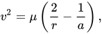
• ${\displaystyle v}$ is the speed of an orbiting body,
• ${\displaystyle \mu =GM}$ is the standard gravitational parameter of the primary body, assuming ${\displaystyle M+m}$ is not significantly bigger than ${\displaystyle M}$ (which makes ${\displaystyle v_{M}\ll v}$), (for Earth, this is μ~3.986E14 m³ s⁻²)
• ${\displaystyle r}$ is the distance of the orbiting body from the primary focus,
• ${\displaystyle a}$ is the semi-major axis of the body's orbit.

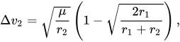
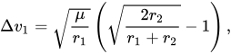
Therefore, the delta-v (Δv) required for the Hohmann transfer can be computed as follows, under the assumption of instantaneous impulses: $${\displaystyle \Delta v_{1}={\sqrt {\frac {\mu }{r_{1}}}}\left({\sqrt {\frac {2r_{2}}{r_{1}+r_{2}}}}-1\right),}$$ to enter the elliptical orbit at ${\displaystyle r=r_{1}}$ from the ${\displaystyle r_{1}}$ circular orbit, where ${\displaystyle r_{2}}$ is the aphelion of the resulting elliptical orbit, and $${\displaystyle \Delta v_{2}={\sqrt {\frac {\mu }{r_{2}}}}\left(1-{\sqrt {\frac {2r_{1}}{r_{1}+r_{2}}}}\right),}$$ to leave the elliptical orbit at ${\displaystyle r=r_{2}}$ to the ${\displaystyle r_{2}}$ circular orbit, where ${\displaystyle r_{1}}$ and ${\displaystyle r_{2}}$ are respectively the radii of the departure and arrival circular orbits; the smaller (greater) of ${\displaystyle r_{1}}$ and ${\displaystyle r_{2}}$ corresponds to the periapsis distance (apoapsis distance) of the Hohmann elliptical transfer orbit. Typically, ${\displaystyle \mu }$ is given in units of m³/s², as such be sure to use meters, not kilometers, for ${\displaystyle r_{1}}$ and ${\displaystyle r_{2}}$. The total ${\displaystyle \Delta v}$ is then:

$${\displaystyle \Delta v_{\text{total}}=\Delta v_{1}+\Delta v_{2}.}$$

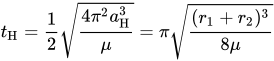
Whether moving into a higher or lower orbit, by Kepler's third law, the time taken to transfer between the orbits is

$${\displaystyle t_{\text{H}}={\frac {1}{2}}{\sqrt {\frac {4\pi ^{2}a_{\text{H}}^{3}}{\mu }}}=\pi {\sqrt {\frac {(r_{1}+r_{2})^{3}}{8\mu }}}}$$ (one half of the orbital period for the whole ellipse), where ${\displaystyle a_{\text{H}}}$ is length of semi-major axis of the Hohmann transfer orbit.

In application to traveling from one celestial body to another it is crucial to start maneuver at the time when the two bodies are properly aligned. Considering the target angular velocity being $${\displaystyle \omega _{2}={\sqrt {\frac {\mu }{r_{2}^{3}}}},}$$ angular alignment α (in radians) at the time of start between the source object and the target object shall be $${\displaystyle \alpha =\pi -\omega _{2}t_{\text{H}}=\pi \left(1-{\frac {1}{2{\sqrt {2}}}}{\sqrt {\left({\frac {r_{1}}{r_{2}}}+1\right)^{3}}}\right).}$$

Consider a geostationary transfer orbit, beginning at r₁ = 6,678 km (altitude 300 km) and ending in a geostationary orbit with r₂ = 42,164 km (altitude 35,786 km).

In the smaller circular orbit the speed is 7.73 km/s; in the larger one, 3.07 km/s. In the elliptical orbit in between the speed varies from 10.15 km/s at the perigee to 1.61 km/s at the apogee.

Therefore the Δv for the first burn is 10.15 − 7.73 = 2.42 km/s, for the second burn 3.07 − 1.61 = 1.46 km/s, and for both together 3.88 km/s.

This is greater than the Δv required for an escape orbit: 10.93 − 7.73 = 3.20 km/s. Applying a Δv at the Low Earth orbit (LEO) of only 0.78 km/s more (3.20−2.42) would give the rocket the escape velocity, which is less than the Δv of 1.46 km/s required to circularize the geosynchronous orbit. This illustrates the Oberth effect that at large speeds the same Δv provides more specific orbital energy, and energy increase is maximized if one spends the Δv as quickly as possible, rather than spending some, being decelerated by gravity, and then spending some more to overcome the deceleration (of course, the objective of a Hohmann transfer orbit is different).

As the example above demonstrates, the Δv required to perform a Hohmann transfer between two circular orbits is not the greatest when the destination radius is infinite. (Escape speed is √2 times orbital speed, so the Δv required to escape is √2 − 1 (41.4%) of the orbital speed.) The Δv required is greatest (53.0% of smaller orbital speed) when the radius of the larger orbit is 15.5817... times that of the smaller orbit.^[10] This number is the positive root of x³ − 15x² − 9x − 1 = 0, which is ${\textstyle 5+4\,{\sqrt {7}}\cos \left({1 \over 3}\arctan {{\sqrt {3}} \over 37}\right)}$. For higher orbit ratios the Δv required for the second burn decreases faster than the first increases.

When used to move a spacecraft from orbiting one planet to orbiting another, the Oberth effect allows to use less delta-v than the sum of the delta-v for separate manoeuvres to escape the first planet, followed by a Hohmann transfer to the second planet, followed by insertion into an orbit around the other planet.

For example, consider a spacecraft travelling from Earth to Mars. At the beginning of its journey, the spacecraft will already have a certain velocity and kinetic energy associated with its orbit around Earth. During the burn the rocket engine applies its delta-v, but the kinetic energy increases as a square law, until it is sufficient to escape the planet's gravitational potential, and then burns more so as to gain enough energy to get into the Hohmann transfer orbit (around the Sun). Because the rocket engine is able to make use of the initial kinetic energy of the propellant, far less delta-v is required over and above that needed to reach escape velocity, and the optimum situation is when the transfer burn is made at minimum altitude (low periapsis) above the planet. The delta-v needed is only 3.6 km/s, only about 0.4 km/s more than needed to escape Earth, even though this results in the spacecraft going 2.9 km/s faster than the Earth as it heads off for Mars (see table below).

At the other end, the spacecraft must decelerate for the gravity of Mars to capture it. This capture burn should optimally be done at low altitude to also make best use of the Oberth effect. Therefore, relatively small amounts of thrust at either end of the trip are needed to arrange the transfer compared to the free space situation.

However, with any Hohmann transfer, the alignment of the two planets in their orbits is crucial – the destination planet and the spacecraft must arrive at the same point in their respective orbits around the Sun at the same time. This requirement for alignment gives rise to the concept of launch windows.

The term lunar transfer orbit (LTO) is used for the Moon.

It is possible to apply the formula given above to calculate the Δv in km/s needed to enter a Hohmann transfer orbit to arrive at various destinations from Earth (assuming circular orbits for the planets). In this table, the column labeled "Δv to enter Hohmann orbit from Earth's orbit" gives the change from Earth's velocity to the velocity needed to get on a Hohmann ellipse whose other end will be at the desired distance from the Sun. The column labeled "LEO height" gives the velocity needed (in a non-rotating frame of reference centered on the earth) when 300 km above the Earth's surface. This is obtained by adding to the specific kinetic energy the square of the escape velocity (10.93 km/s) from this height. The column "LEO" is simply the previous speed minus the LEO orbital speed of 7.73 km/s.

Note that in most cases, Δv from LEO is less than the Δv to enter Hohmann orbit from Earth's orbit.

To get to the Sun, it is actually not necessary to use a Δv of 24 km/s. One can use 8.8 km/s to go very far away from the Sun, then use a negligible Δv to bring the angular momentum to zero, and then fall into the Sun. This is also known as a bi-elliptic transfer, which is a sequence of two Hohmann transfers. Also, the table does not give the values that would apply when using the Moon for a gravity assist. There are also possibilities of using one planet, like Venus which is the easiest to get to, to assist getting to other planets or the Sun.

The bi-elliptic transfer consists of two half-elliptic orbits. From the initial orbit, a first burn expends delta-v to boost the spacecraft into the first transfer orbit with an apoapsis at some point ${\displaystyle r_{b}}$ away from the central body. At this point a second burn sends the spacecraft into the second elliptical orbit with periapsis at the radius of the final desired orbit, where a third burn is performed, injecting the spacecraft into the desired orbit.^[11]

While they require one more engine burn than a Hohmann transfer and generally require a greater travel time, some bi-elliptic transfers require a lower amount of total delta-v than a Hohmann transfer when the ratio of final to initial semi-major axis is 11.94 or greater, depending on the intermediate semi-major axis chosen.^[12]

The idea of the bi-elliptical transfer trajectory was first^{[citation needed]} published by Ary Sternfeld in 1934.^[13]

Low-thrust engines can perform an approximation of a Hohmann transfer orbit, by creating a gradual enlargement of the initial circular orbit through carefully timed engine firings. This requires a change in velocity (delta-v) that is greater than the two-impulse transfer orbit^[14] and takes longer to complete.

Engines such as ion thrusters are more difficult to analyze with the delta-v model. These engines offer a very low thrust and at the same time, much higher delta-v budget, much higher specific impulse, lower mass of fuel and engine. A 2-burn Hohmann transfer maneuver would be impractical with such a low thrust; the maneuver mainly optimizes the use of fuel, but in this situation there is relatively plenty of it.

If only low-thrust maneuvers are planned on a mission, then continuously firing a low-thrust, but very high-efficiency engine might generate a higher delta-v and at the same time use less propellant than a conventional chemical rocket engine.

Going from one circular orbit to another by gradually changing the radius simply requires the same delta-v as the difference between the two speeds.^[14] Such maneuver requires more delta-v than a 2-burn Hohmann transfer maneuver, but does so with continuous low thrust rather than the short applications of high thrust.

The amount of propellant mass used measures the efficiency of the maneuver plus the hardware employed for it. The total delta-v used measures the efficiency of the maneuver only. For electric propulsion systems, which tend to be low-thrust, the high efficiency of the propulsive system usually compensates for the higher delta-V compared to the more efficient Hohmann maneuver.

Transfer orbits using electrical propulsion or low-thrust engines optimize the transfer time to reach the final orbit and not the delta-v as in the Hohmann transfer orbit. For geostationary orbit, the initial orbit is set to be supersynchronous and by thrusting continuously in the direction of the velocity at apogee, the transfer orbit transforms to a circular geosynchronous one. This method however takes much longer to achieve due to the low thrust injected into the orbit.^[15]

In 1997, a set of orbits known as the Interplanetary Transport Network (ITN) was published, providing even lower propulsive delta-v (though much slower and longer) paths between different orbits than Hohmann transfer orbits.^[16] The Interplanetary Transport Network is different in nature than Hohmann transfers because Hohmann transfers assume only one large body whereas the Interplanetary Transport Network does not. The Interplanetary Transport Network is able to achieve the use of less propulsive delta-v by employing gravity assist from the planets.^{[citation needed]}

• Bi-elliptic transfer
• Delta-v budget
• Geostationary transfer orbit
• Halo orbit
• Lissajous orbit
• List of orbits
• Orbital mechanics

• Bate, R. R.; Mueller, D.D.; White, J.E. (1971). Fundamentals of Astrodynamics. New York: Dover Publications. ISBN 978-0-486-60061-1.
• Battin, R .H. (1999). An Introduction to the Mathematics and Methods of Astrodynamics. Washington, DC: American Institute of Aeronautics & Ast. ISBN 978-1-56347-342-5.
• Hohmann, Walter (1994) [1925]. Die Erreichbarkeit der Himmelskörper. Munich: R. Oldenbourg Verlag. ISBN 3-486-23106-5.
• Thornton, Stephen T.; Marion, Jerry B. (2003). Classical Dynamics of Particles and Systems (5th ed.). Brooks Cole. ISBN 0-534-40896-6.
• Vallado, D. A. (2001). Fundamentals of Astrodynamics and Applications (2nd ed.). Springer. ISBN 978-0-7923-6903-5.