Hubbry Logo
search
logo
2221212

State function

logo
Community Hub0 Subscribers
Read side by side
from Wikipedia

In the thermodynamics of equilibrium, a state function, function of state, or point function for a thermodynamic system is a mathematical function relating several state variables or state quantities (that describe equilibrium states of a system) that depend only on the current equilibrium thermodynamic state of the system[1] (e.g. gas, liquid, solid, crystal, or emulsion), not the path which the system has taken to reach that state. A state function describes equilibrium states of a system, thus also describing the type of system. A state variable is typically a state function so the determination of other state variable values at an equilibrium state also determines the value of the state variable as the state function at that state. The ideal gas law is a good example. In this law, one state variable (e.g., pressure, volume, temperature, or the amount of substance in a gaseous equilibrium system) is a function of other state variables so is regarded as a state function. A state function could also describe the number of a certain type of atoms or molecules in a gaseous, liquid, or solid form in a heterogeneous or homogeneous mixture, or the amount of energy required to create such a system or change the system into a different equilibrium state.

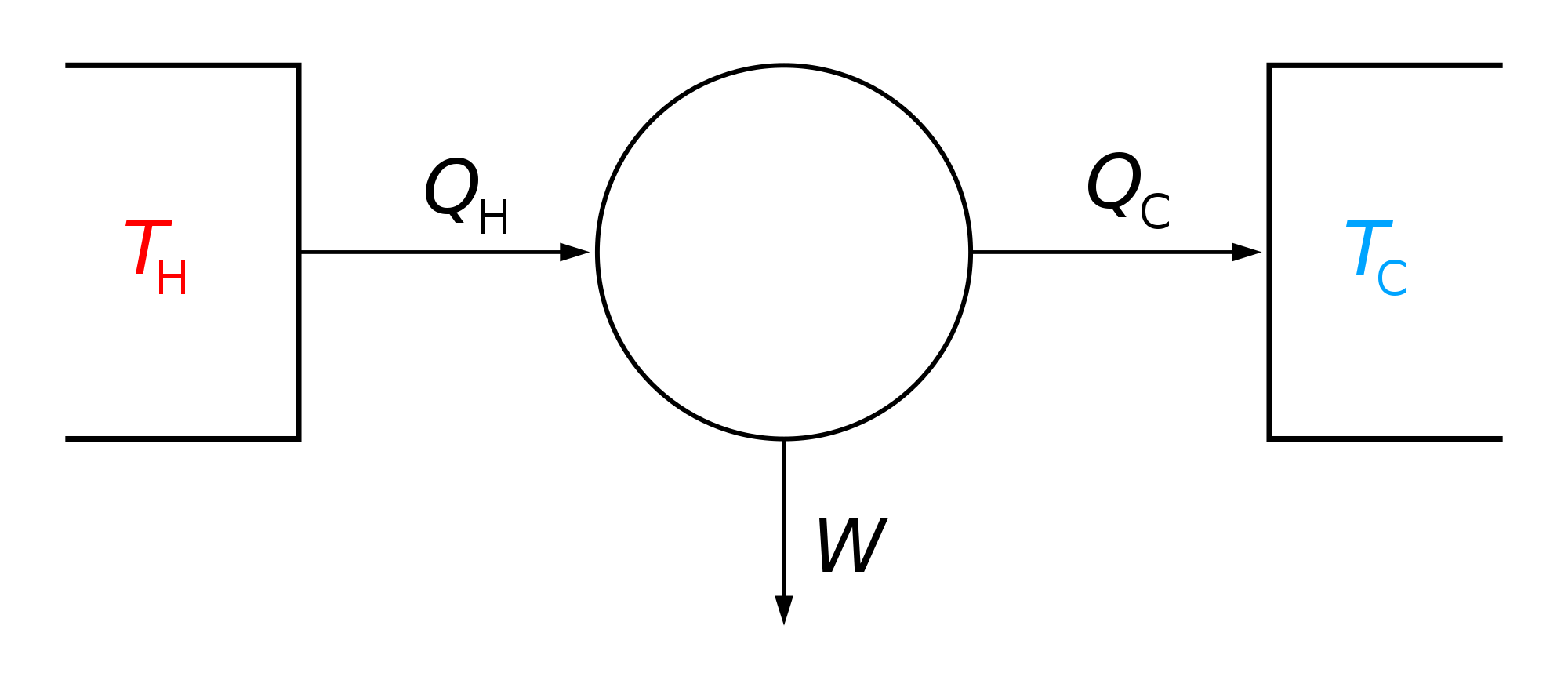
Internal energy, enthalpy, and entropy are examples of state quantities or state functions because they quantitatively describe an equilibrium state of a thermodynamic system, regardless of how the system has arrived in that state. They are expressed by exact differentials. In contrast, mechanical work and heat are process quantities or path functions because their values depend on a specific "transition" (or "path") between two equilibrium states that a system has taken to reach the final equilibrium state, being expressed by inexact differentials. Exchanged heat (in certain discrete amounts) can be associated with changes of state function such as enthalpy. The description of the system heat exchange is done by a state function, and thus enthalpy changes point to an amount of heat. This can also apply to entropy when heat is compared to temperature. The description breaks down for quantities exhibiting hysteresis.[2]

History

[edit]

It is likely that the term "functions of state" was used in a loose sense during the 1850s and 1860s by those such as Rudolf Clausius, William Rankine, Peter Tait, and William Thomson. By the 1870s, the term had acquired a use of its own. In his 1873 paper "Graphical Methods in the Thermodynamics of Fluids", Willard Gibbs states: "The quantities v, p, t, ε, and η are determined when the state of the body is given, and it may be permitted to call them functions of the state of the body."[3]

Overview

[edit]

A thermodynamic system is described by a number of thermodynamic parameters (e.g. temperature, volume, or pressure) which are not necessarily independent. The number of parameters needed to describe the system is the dimension of the state space of the system (D). For example, a monatomic gas with a fixed number of particles is a simple case of a two-dimensional system (D = 2). Any two-dimensional system is uniquely specified by two parameters. Choosing a different pair of parameters, such as pressure and volume instead of pressure and temperature, creates a different coordinate system in two-dimensional thermodynamic state space but is otherwise equivalent. Pressure and temperature can be used to find volume, pressure and volume can be used to find temperature, and temperature and volume can be used to find pressure. An analogous statement holds for higher-dimensional spaces, as described by the state postulate.

Generally, a state space is defined by an equation of the form , where P denotes pressure, T denotes temperature, V denotes volume, and the ellipsis denotes other possible state variables like particle number N and entropy S. If the state space is two-dimensional as in the above example, it can be visualized as a three-dimensional graph (a surface in three-dimensional space). However, the labels of the axes are not unique (since there are more than three state variables in this case), and only two independent variables are necessary to define the state.

When a system changes state continuously, it traces out a "path" in the state space. The path can be specified by noting the values of the state parameters as the system traces out the path, whether as a function of time or a function of some other external variable. For example, having the pressure P(t) and volume V(t) as functions of time from time t0 to t1 will specify a path in two-dimensional state space. Any function of time can then be integrated over the path. For example, to calculate the work done by the system from time t0 to time t1, calculate . In order to calculate the work W in the above integral, the functions P(t) and V(t) must be known at each time t over the entire path. In contrast, a state function only depends upon the system parameters' values at the endpoints of the path. For example, the following equation can be used to calculate the work plus the integral of V dP over the path:

In the equation, can be expressed as the exact differential of the function P(t)V(t). Therefore, the integral can be expressed as the difference in the value of P(t)V(t) at the end points of the integration. The product PV is therefore a state function of the system.

The notation d will be used for an exact differential. In other words, the integral of dΦ will be equal to Φ(t1) − Φ(t0). The symbol δ will be reserved for an inexact differential, which cannot be integrated without full knowledge of the path. For example, δW = PdV will be used to denote an infinitesimal increment of work.

State functions represent quantities or properties of a thermodynamic system, while non-state functions represent a process during which the state functions change. For example, the state function PV is proportional to the internal energy of an ideal gas, but the work W is the amount of energy transferred as the system performs work. Internal energy is identifiable; it is a particular form of energy. Work is the amount of energy that has changed its form or location.

List of state functions

[edit]

The following are considered to be state functions in thermodynamics:

See also

[edit]

Notes

[edit]

References

[edit]
[edit]
Revisions and contributorsEdit on WikipediaRead on Wikipedia
from Grokipedia
In thermodynamics, a state function is a property of a thermodynamic system that depends solely on the current equilibrium state of the system, regardless of the history or path by which that state was reached.[1] Unlike path functions such as heat and work, which vary depending on the specific process undergone, state functions ensure that changes in their values (e.g., ΔU for internal energy) are identical for any process connecting the same initial and final states.[2] This path-independence is fundamental to the first law of thermodynamics, where the change in internal energy equals the sum of heat and work, but only the internal energy change is uniquely determined by the endpoints.[3] Common examples of state functions include internal energy (U), which represents the total kinetic and potential energy of the system's particles; enthalpy (H), defined as H = U + PV and useful for constant-pressure processes; entropy (S), a measure of disorder or randomness that drives spontaneity; Gibbs free energy (G = H - TS), which predicts reaction feasibility at constant temperature and pressure; and basic variables like temperature (T), pressure (P), and volume (V).[4][5][6] These properties are either extensive (scaling with system size, like U and V) or intensive (independent of size, like T and P), enabling precise characterization of macroscopic behavior from microscopic interactions.[7] The concept extends to all thermodynamic properties, facilitating equilibrium analysis, cycle efficiency calculations in engines, and phase behavior predictions in materials science.[8]

Fundamentals

Definition and Core Properties

In thermodynamics and physical sciences, a state function is defined as a property of a system that depends solely on its current equilibrium state, rather than on the history or the specific process by which that state was achieved. This means that for any given set of state variables—such as pressure, volume, and temperature—the value of a state function remains the same regardless of the path taken to reach that configuration. The equilibrium state itself is characterized by a complete specification of these variables, ensuring the system is uniform and stable, with no ongoing changes or gradients.[9] Core properties of state functions reflect the smooth, continuous nature of equilibrium configurations. Extensive state functions exhibit additivity when considering composite systems, meaning the total value for the combined system is the sum of the values for each subsystem, provided the subsystems are in mutual equilibrium.[4] In isolated systems, certain state functions such as internal energy are conserved, maintaining constant values.[10] To illustrate conceptually, consider the height of a point on a mountain: this elevation is a state function because it depends only on the current position (the state), not on whether one ascended via a steep trail or a gentle slope. This analogy underscores the path-independence inherent to state functions, emphasizing their utility in predicting system behavior without tracing every possible trajectory.

Distinction from Path Functions

Path functions, in contrast to state functions, are thermodynamic properties whose values depend on the specific path or process taken to transition between states of a system, rather than solely on the initial and final states. Classic examples include heat (Q) and work (W), which vary according to the trajectory of the process, such as the manner of compression or expansion in a thermodynamic cycle.[5] The fundamental criterion distinguishing state functions from path functions lies in path independence: for a state function Z, the change ΔZ is given by ΔZ = Zfinal - Zinitial, independent of the path taken, whereas for path functions, the change is path-dependent and expressed as the line integral ∫đpath along the specific trajectory.[11] This distinction arises because state functions correspond to exact differentials, while path functions involve inexact differentials that cannot be integrated without specifying the process details.[6] A practical test for identifying state functions is the cycle integral criterion: for a state function Z, the line integral around any closed thermodynamic cycle is zero, ∮dZ = 0, reflecting the return to the initial state without net change, whereas for path functions, this integral is generally nonzero.[12] This test, rooted in the properties of conservative fields in thermodynamics, confirms path independence by ensuring no residual dependence on the cycle's trajectory.[13] The distinction between state and path functions has significant implications for thermodynamic analysis, as it allows changes in state functions to be computed efficiently using only initial and final states, bypassing the need for detailed path-specific integrations that are required for path functions.[8] This efficiency underpins the first law of thermodynamics, where the state function internal energy U balances the path-dependent heat and work, enabling broader applications in process design and energy accounting without exhaustive process simulations.[14]

Historical Context

Origins in Thermodynamics

The conceptual foundations of state functions in thermodynamics took shape during the Industrial Revolution, amid efforts to improve the efficiency of steam engines and other heat engines that powered emerging industries. French engineer Sadi Carnot's 1824 publication, Réflexions sur la puissance motrice du feu et sur les machines propres à développer cette puissance, provided an early theoretical framework by analyzing the maximum efficiency of heat engines operating between two temperatures. Although Carnot adhered to the caloric theory of heat as a conserved fluid, his derivation of engine efficiency as a fixed ratio dependent solely on the source and sink temperatures implicitly invoked path-independent quantities, as the work output in ideal reversible cycles did not vary with the specific sequence of processes.[15] This period also witnessed the erosion of the caloric theory, which had dominated since the 18th century by treating heat as an indestructible, weightless fluid that could be transferred but not created or destroyed. Experiments by Benjamin Thompson, Count Rumford, in 1798 demonstrated that boring cannon barrels generated unlimited heat through friction without any evident depletion of caloric, suggesting heat arose from mechanical motion rather than a conserved substance. Further evidence came from Humphry Davy's 1799 ice-melting experiments and James Prescott Joule's precise measurements in the 1840s, which quantified the mechanical equivalent of heat and showed heat production proportional to work done, undermining caloric conservation. These findings propelled the mechanical theory of heat, advanced by Julius Robert von Mayer and Hermann von Helmholtz, which equated heat to molecular motion and emphasized conserved quantities like vis viva (later energy), setting the stage for path-independent state descriptions in thermodynamic systems.[16][17] Rudolf Clausius built directly on this shift in the 1850s, formalizing the first law of thermodynamics and introducing internal energy as a key conserved quantity. In his seminal 1850 memoir, Über die bewegende Kraft der Wärme (On the Moving Force of Heat), Clausius argued that for cyclic processes, the total heat absorbed equals the work performed, implying the existence of a state quantity—internal energy—whose change between two states is independent of the path connecting them. This path independence arose from equating heat and work as interchangeable forms of a single conserved energy, resolving inconsistencies in earlier theories and establishing internal energy as the first explicit thermodynamic state function. Clausius did not initially employ the modern term "state function," but by 1865, in his paper Über mehrere für die Anwendung bequeme Formen der fundamentalen Gleichungen der mechanischen Wärmetheorie (On Several Convenient Forms of the Fundamental Equations of the Mechanical Theory of Heat), he explicitly described quantities like internal energy and the newly introduced entropy as "functions of state," determined solely by the system's condition at a given moment. This terminology underscored their path independence, contrasting with path-dependent quantities like work and heat, and solidified the recognition of conserved, state-determined properties amid the mechanical theory's triumph over caloric ideas.[18]

Key Developments and Contributors

The development of state function theory in thermodynamics owes much to Rudolf Clausius, who in 1865 formalized entropy as a state function integral to the second law of thermodynamics. In his paper "On Several Convenient Forms of the Fundamental Equations of the Mechanical Theory of Heat," Clausius defined entropy S such that its change dS = δQ_rev / T for reversible processes, emphasizing its path-independence and dependence solely on the system's equilibrium states, thereby establishing it as a fundamental measure of disorder or unavailable energy.[18] Josiah Willard Gibbs emerged as a central figure in the late 1870s, introducing enthalpy, Helmholtz free energy, and Gibbs free energy as state functions within chemical thermodynamics. In his landmark publication "On the Equilibrium of Heterogeneous Substances" (1876–1878), Gibbs defined the Helmholtz free energy A = U - TS (where U is internal energy, T temperature, and S entropy) for processes at constant temperature and volume, and the Gibbs free energy G = A + PV (with PV as pressure-volume work, equivalent to H - TS where H = U + PV represents the enthalpy or heat content at constant pressure) for constant temperature and pressure conditions; these potentials determine spontaneity and equilibrium by minimization. Gibbs also formulated the phase rule F = C - P + 2 (where F is degrees of freedom, C components, and P phases), relying on state functions to predict the variability of heterogeneous systems at equilibrium. Although Gibbs did not coin "enthalpy," he operationalized H as a state function crucial for constant-pressure processes.[19][20] In the late 19th century, Ludwig Boltzmann and James Clerk Maxwell advanced the microscopic foundations of state functions through statistical mechanics. Maxwell's 1867 paper "On the Dynamical Theory of Gases" developed the velocity distribution in ideal gases via kinetic theory, linking macroscopic properties like pressure and temperature to averages over molecular states without path dependence in equilibrium. Boltzmann built on this in his 1877 work "Über die Beziehung zwischen dem zweiten Hauptsatz der mechanischen Wärmetheorie und der Wahrscheinlichkeitsrechnung," connecting entropy to microscopic configurations via S = k ln W (k Boltzmann's constant, W number of microstates), demonstrating that state functions emerge as equilibrium-independent quantities from probabilistic ensembles of microscopic states.[21][22] Max Planck contributed significantly around 1900 by incorporating quantum effects into energy states, influencing the statistical mechanics of state functions. In his 1900 derivation of blackbody radiation law, Planck quantized oscillator energies as E = nhf (n integer, h Planck's constant, f frequency), resolving the ultraviolet catastrophe and enabling a discrete treatment of microscopic states that refined the path-independent nature of thermodynamic potentials in quantum systems.[23] Ilya Prigogine refined state function concepts for non-equilibrium systems from the 1940s to 1960s, extending their applicability beyond classical equilibrium thermodynamics. In "Introduction to Thermodynamics of Irreversible Processes" (1955) and subsequent works, Prigogine introduced local state functions under the local equilibrium hypothesis, where variables like temperature and entropy are defined instantaneously in small volumes; he distinguished these from global states and developed the minimum entropy production principle for near-equilibrium steady states, while later advancing dissipative structures where far-from-equilibrium systems exhibit ordered patterns driven by irreversible processes.

Mathematical Representation

State Variables and Systems

State variables are the independent thermodynamic properties, such as pressure PP, volume VV, temperature TT, and the number of moles nn, that collectively specify the macroscopic state of a system in thermodynamic equilibrium.[24] These variables must be sufficient in number and choice to uniquely determine all other thermodynamic properties of the system, ensuring that the state is fully described without ambiguity.[1] In practice, for a simple gas, specifying PP, VV, and TT often suffices, though additional variables like composition may be needed for multicomponent systems.[4] Thermodynamic systems are classified based on their interactions with the surroundings, which influences how state functions behave.[25] A closed system exchanges energy but not matter with its surroundings, allowing state functions like internal energy to change via heat or work while volume remains fixed if rigid.[26] An open system permits both matter and energy exchange, complicating state function tracking due to mass flow, though variables like PP and TT still define local equilibrium states.[27] In an isolated system, neither matter nor energy is exchanged, so state functions such as total energy and volume remain constant, preserving the system's state over time.[28] The concept of state space provides a geometric framework for understanding states, visualized as a multidimensional space where each axis corresponds to a state variable and every point represents a unique equilibrium state of the system.[29] In this space, state functions can be represented as coordinates defining the position or as surfaces where the function holds constant values, such as isotherms in the PP-VV-TT space.[30] This abstraction highlights the path independence of state functions, as the value at any point depends solely on the coordinates, not the route taken to reach it.[4] The number of independent state variables required is determined by the degrees of freedom, quantified by the Gibbs phase rule: $ F = C - P + 2 $, where $ F $ is the degrees of freedom, $ C $ the number of components, and $ P $ the number of phases.[31] This rule indicates the minimal set of variables needed to specify the state; for a single-component, single-phase system like an ideal gas, $ F = 2 $, so two variables (e.g., $ P $ and $ T )sufficeviatheequationofstate.[](https://serc.carleton.edu/researcheducation/equilibria/phaserule.html)Inmultiphasesystems,suchasaliquidvaporequilibrium() suffice via the equation of state.[](https://serc.carleton.edu/research_education/equilibria/phaserule.html) In multiphase systems, such as a liquid-vapor equilibrium ( P = 2 $), $ F = 1 $, fixing one variable like $ T $ determines the rest, underscoring the rule's role in state specification.[32]

Exact and Inexact Differentials

In thermodynamics, the differential of a state function ZZ, such as internal energy or entropy, is an exact differential, expressed as
dZ=(Zx)ydx+(Zy)xdy, dZ = \left( \frac{\partial Z}{\partial x} \right)_y \, dx + \left( \frac{\partial Z}{\partial y} \right)_x \, dy,
where xx and yy are state variables, and the change in ZZ depends only on the initial and final states, not the path taken between them.[33][34] This path independence implies that the line integral of dZdZ over any closed path is zero, dZ=0\oint dZ = 0.[33] A key mathematical property ensuring exactness is the integrability condition, derived from multivariable calculus, which states that the mixed second partial derivatives must be equal:
2Zxy=2Zyx. \frac{\partial^2 Z}{\partial x \partial y} = \frac{\partial^2 Z}{\partial y \partial x}.
This condition guarantees that dZdZ is the total differential of a single-valued function ZZ.[34][35] In contrast, differentials of path functions, such as heat transfer δQ\delta Q or work δW\delta W, are inexact, typically written as δZ=Mdx+Ndy\delta Z = M \, dx + N \, dy, where the cross-partial derivatives do not satisfy M/y=N/x\partial M / \partial y = \partial N / \partial x.[33][36] As a result, the integral δZ0\oint \delta Z \neq 0 in general, reflecting path dependence; for instance, the work done in a thermodynamic cycle varies with the process route.[33] The first law of thermodynamics illustrates this distinction clearly:
dU=δQ+δW, dU = \delta Q + \delta W,
where dUdU is the exact differential of the state function internal energy UU, while δQ\delta Q and δW\delta W are inexact differentials of path-dependent quantities.[35][36] This equation shows how the path-independent change in UU arises from the sum of path-dependent heat and work.[35] To identify whether a differential form is exact in thermodynamic systems, one employs tests from the theory of Pfaffian differential equations, which are linear forms of the type ω=M(x,y)dx+N(x,y)dy\omega = M(x,y) \, dx + N(x,y) \, dy.[35] The primary test for exactness is the equality of the mixed partials, M/y=N/x\partial M / \partial y = \partial N / \partial x, confirming integrability.[33][34] If this holds, ω=dZ\omega = dZ for some state function ZZ; otherwise, an integrating factor may exist to render it exact, though in thermodynamics, inexact forms like δW=PdV\delta W = -P \, dV often lack such factors without additional constraints.[35] For multivariable cases, Euler's criterion generalizes this: for ω=iMidxi\omega = \sum_i M_i \, dx_i, exactness requires Mi/xj=Mj/xi\partial M_i / \partial x_j = \partial M_j / \partial x_i for all pairs i,ji,j.[34] These tests are essential for deriving thermodynamic relations, such as Maxwell's equations, from the exactness of state function differentials.[35]

Common Examples

Thermodynamic State Functions

In classical thermodynamics, state functions, also known as thermodynamic potentials, are extensive properties that depend solely on the equilibrium state of the system, independent of the path taken to reach that state. These functions are crucial for describing energy transformations and equilibrium conditions in physical and chemical systems. The primary thermodynamic state functions are internal energy, enthalpy, Helmholtz free energy, Gibbs free energy, and entropy, each expressed as a function of natural variables such as temperature $ T $, pressure $ P $, volume $ V $, and entropy $ S $. Their differential forms, derived from the first and second laws of thermodynamics, facilitate the analysis of reversible processes. The internal energy $ U(S, V) $ is the total microscopic energy content of the system, encompassing kinetic and potential energies of its constituents. For reversible processes involving heat and pressure-volume work, the fundamental relation is given by
dU=TdSPdV, dU = T \, dS - P \, dV,
where $ T $ is the absolute temperature and $ P $ is the pressure.[37] This expression highlights $ U $ as a function of entropy and volume, with $ T $ and $ -P $ as the conjugate variables. Enthalpy $ H $, defined as $ H = U + P V $, extends the internal energy to account for pressure-volume contributions, making it particularly useful for processes at constant pressure. Its differential form is
dH=TdS+VdP, dH = T \, dS + V \, dP,
positioning $ H $ as a natural function of $ S $ and $ P $, with $ T $ and $ V $ as conjugates.[37] The Helmholtz free energy $ A $ (often denoted $ F $), given by $ A = U - T S $, represents the maximum work extractable from a system at constant temperature and volume, excluding expansion work. Its differential is
dA=SdTPdV, dA = -S \, dT - P \, dV,
indicating $ A(T, V) $ as the potential, with $ -S $ and $ -P $ as response functions.[37] The Gibbs free energy $ G $, defined as $ G = H - T S $ or equivalently $ G = U + P V - T S $, is the key potential for processes at constant temperature and pressure, such as chemical reactions. The relation is
dG=SdT+VdP, dG = -S \, dT + V \, dP,
with $ G(T, P) $ and conjugates $ -S $ and $ V $.[37] Entropy $ S $ quantifies the dispersal of energy or the degree of molecular disorder within the system. For a reversible process, it is defined by the relation
dS=δQrevT, dS = \frac{\delta Q_{\rm rev}}{T},
where $ \delta Q_{\rm rev} $ is the infinitesimal reversible heat transfer.[38] This makes $ S $ an extensive state function that increases in isolated systems, reflecting the second law of thermodynamics.[39] These thermodynamic potentials are interconnected via Legendre transforms, which systematically change the independent variables from extensive to intensive ones (or vice versa) while preserving the underlying physics. For instance, the transform from $ U(S, V) $ to enthalpy is $ H(S, P) = U + P V $, incorporating the conjugate pair $ (V, P) $; similarly, $ A(T, V) = U - T S $ transforms $ (S, T) $, and $ G(T, P) = U + P V - T S $ combines both.[37] These relations ensure consistency across different ensembles and experimental conditions in thermodynamic analyses.

State Functions in Other Fields

In classical mechanics, state functions describe the configuration of a system in phase space, where the position coordinates and momenta fully specify the state. Position serves as a state function because it depends only on the instantaneous coordinates of the particles, independent of the path taken to reach that configuration. Similarly, potential energy is a state function in conservative systems, determined solely by the positions of the particles, such as gravitational or electrostatic potentials. Kinetic energy, expressed as a function of momenta in the Hamiltonian formalism, also qualifies as a state function within phase space, as it relies exclusively on the current momentum values rather than the history of motion.[40][41][42] In fluid dynamics, particularly for equilibrium or steady-state flows, pressure and density act as state functions that characterize the local thermodynamic state of the fluid. Pressure in a static or hydrostatic fluid is determined by the overlying fluid column's weight and density, following the hydrostatic equation $ dp/dz = -\rho g $, where the pressure gradient with respect to height z equals the negative product of density $ \rho $ and gravitational acceleration $ g $, ensuring path independence from the surface. Density, in turn, reflects the fluid's mass per unit volume at equilibrium, varying with local conditions like temperature and pressure but fixed for a given state without dependence on flow history. These properties enable the description of equilibrium flows where the system returns to the same state regardless of the approach path.[43][44][45] In chemistry, the chemical potential μi\mu_i for a species ii in a mixture is a state function defined as the partial molar Gibbs free energy, given by
μi=(Gni)T,P,nj \mu_i = \left( \frac{\partial G}{\partial n_i} \right)_{T,P,n_j}
where GG is the Gibbs free energy, nin_i is the number of moles of species ii, and the derivative is taken at constant temperature TT, pressure PP, and moles of other species njn_j. This quantity depends only on the composition, temperature, and pressure of the system at equilibrium, making it path-independent and crucial for predicting phase behavior and reaction equilibria in multicomponent systems.[46][47][48] Quantum mechanics extends the notion of state functions to the eigenvalues of operators, such as the energy eigenvalues of the Hamiltonian, which are determined solely by the quantum numbers specifying the system's state. For instance, in the hydrogen atom, the energy eigenvalues depend only on the principal quantum number nn, yielding discrete levels En=13.6n2E_n = -\frac{13.6}{n^2} eV, independent of the quantum state's evolutionary path. These energy levels, as functions of quantum numbers like nn, ll, and mlm_l, fully characterize bound states in quantum systems, such as atomic orbitals, without reliance on transitional dynamics.[49][50][51] More generally, state functions encompass properties of conservative fields, where the associated vector field is the gradient of a scalar potential that depends only on position. In electrostatics, the electric potential ϕ\phi exemplifies this, as the work to move a charge between points is path-independent, with ϕ\phi determined by the charge distribution via Poisson's equation 2ϕ=ρ/ϵ0\nabla^2 \phi = -\rho / \epsilon_0. Such potentials in irrotational fields (×F=0\nabla \times \mathbf{F} = 0) ensure that the field's line integral is solely a function of endpoints, mirroring the path independence central to state functions across physical sciences.[52][53][54]

Applications and Implications

Role in Thermodynamic Processes

State functions play a pivotal role in analyzing thermodynamic processes by depending solely on the initial and final states of a system, rather than the specific path traversed. This path independence means that changes in state functions, such as internal energy (ΔU\Delta U) and enthalpy (ΔH\Delta H), can be computed directly from the properties of the starting and ending states, simplifying the evaluation of energy transformations without needing details of intermediate steps. For instance, in processes like the Carnot cycle, this property allows engineers and physicists to focus on endpoint conditions to determine overall energy balances.[55][56] In closed thermodynamic cycles, where the system returns to its original state, state functions exhibit zero net change, providing a foundational tool for cycle analysis. This implies ΔU=0\Delta U = 0 for the entire cycle, and from the first law of thermodynamics, the cyclic integrals satisfy δQ=δW\oint \delta Q = -\oint \delta W, relating the total heat absorbed to the net work output independently of the cycle's internal details. Such cycles, exemplified by the Carnot cycle, leverage this to assess efficiency and energy conversion without path-specific calculations.[57][56] State functions also serve as criteria for equilibrium and spontaneity in thermodynamic processes. The Gibbs free energy (GG), a key state function, predicts spontaneity at constant temperature and pressure: a process is spontaneous if ΔG<0\Delta G < 0, at equilibrium if ΔG=0\Delta G = 0, and non-spontaneous if ΔG>0\Delta G > 0. This is particularly evident in phase transitions, where ΔG=0\Delta G = 0 marks the boundary between phases, such as liquid-vapor equilibrium.[58][59] Regardless of whether a process is reversible or irreversible, the change in any state function remains identical, as it is determined only by the endpoint states. However, path functions like heat (QQ) and work (WW) vary: for irreversible processes, the actual heat exchanged (QQ) is typically less than the reversible heat (QrevQ_\text{rev}), reflecting inefficiencies such as friction or rapid changes. This distinction enables the use of reversible path assumptions to compute state function changes accurately, even for real-world irreversible scenarios.[60]

Importance in Engineering and Physics

In engineering applications such as heat engines, refrigeration cycles, and chemical reactors, state functions like internal energy, enthalpy, and entropy enable precise predictions of system efficiency by depending solely on initial and final states, independent of the path taken. For instance, in heat engines operating on cyclic processes, the net change in internal energy is zero (ΔU = 0), allowing efficiency to be calculated as the ratio of work output to heat input, with the Carnot efficiency serving as the theoretical maximum: η = 1 - (T_c / T_h), where T_h and T_c are the hot and cold reservoir temperatures in Kelvin.[61] This derivation relies on the reversibility condition where the total entropy change is zero (ΔS = 0) across the cycle, facilitating design optimizations for devices like steam turbines or internal combustion engines.[7] Similarly, in refrigeration systems, the coefficient of performance (COP) for an ideal Carnot refrigerator is derived from state functions as COP = T_c / (T_h - T_c), again using ΔS = 0 to bound the heat extracted from the cold reservoir relative to work input, guiding the development of efficient vapor-compression cycles.[62] In chemical reactors, state functions such as Gibbs free energy determine reaction spontaneity and equilibrium yields under varying conditions, enabling process simulations that minimize energy waste in industrial synthesis.[7] State functions are integral to physical modeling in computational simulations, particularly in computational fluid dynamics (CFD), where variables like pressure, temperature, and density define fluid states to solve conservation equations for mass, momentum, and energy. Accurate representation of these state variables through empirical correlations or steam tables enhances the fidelity of simulations for complex flows, such as those in aerospace or HVAC systems, by capturing thermodynamic properties without path-dependent errors.[63] This approach allows engineers to predict phenomena like turbulence or heat transfer in steady-state or transient conditions, reducing reliance on experimental trials and improving design iterations.[64] Beyond core engineering, state functions underpin broader impacts in sustainability through exergy analysis, which quantifies the useful work potential of energy relative to a reference environment using balances of enthalpy, entropy, and other state properties to identify irreversibilities and losses. In building systems, for example, exergy-based evaluations promote low-exergy designs like passive solar heating, reducing consumption from 148 W to 78 W per unit while aligning with environmental goals.[65] In non-equilibrium thermodynamics applied to biological systems, state functions such as free energy dissipation maintain steady states in living processes, like metabolic networks, by coupling energy flows to counteract entropy production in far-from-equilibrium conditions.[66] Modern extensions of state functions appear in nanotechnology and materials science, where Gibbs free energy models phase transitions under extreme conditions, such as high pressure, to predict stability and transformations in nanomaterials. For copper, high-pressure Gibbs energy distributions reveal the stability of a metastable body-centered tetragonal phase under dynamic loading conditions, informing the synthesis of advanced alloys for electronics or catalysis.[67] High-throughput computational methods further leverage Gibbs energy landscapes to map pressure-temperature phase diagrams for multinary solids, accelerating the discovery of materials with tunable properties under nanoconfinement or extreme environments.[68]

References

User Avatar
No comments yet.