Isentropic process

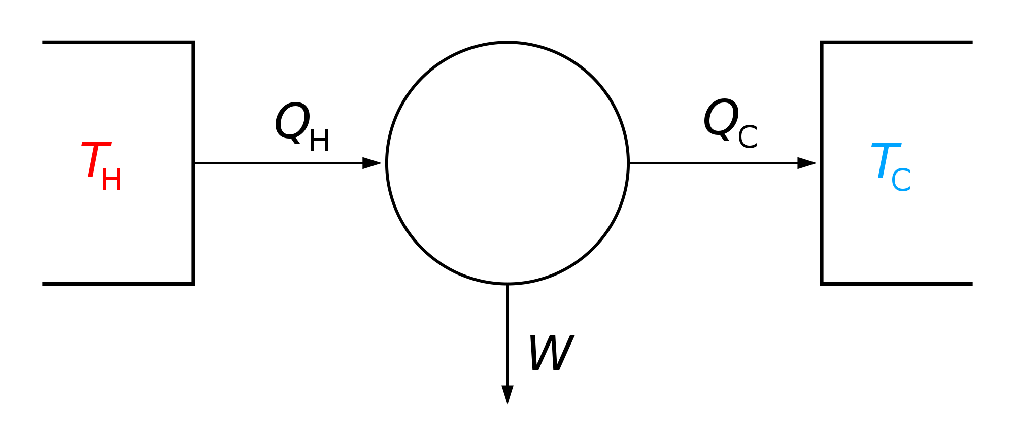
The second law of thermodynamics states^[9][10] that

${\displaystyle T_{\text{surr}}dS\geq \delta Q,}$

where ${\displaystyle \delta Q}$ is the amount of energy the system gains by heating, ${\displaystyle T_{\text{surr}}}$ is the temperature of the surroundings, and ${\displaystyle dS}$ is the change in entropy. The equal sign refers to a reversible process, which is an imagined idealized theoretical limit, never actually occurring in physical reality, with essentially equal temperatures of system and surroundings.^[11][12] For an isentropic process, if also reversible, there is no transfer of energy as heat because the process is adiabatic; δQ = 0. In contrast, if the process is irreversible, entropy is produced within the system; consequently, in order to maintain constant entropy within the system, energy must be simultaneously removed from the system as heat.

For reversible processes, an isentropic transformation is carried out by thermally "insulating" the system from its surroundings. Temperature is the thermodynamic conjugate variable to entropy, thus the conjugate process would be an isothermal process, in which the system is thermally "connected" to a constant-temperature heat bath.

The entropy of a given mass does not change during a process that is internally reversible and adiabatic. A process during which the entropy remains constant is called an isentropic process, written ${\displaystyle \Delta s=0}$ or ${\displaystyle s_{1}=s_{2}}$.^[13] Some examples of theoretically isentropic thermodynamic devices are pumps, gas compressors, turbines, nozzles, and diffusers.

Most steady-flow devices operate under adiabatic conditions, and the ideal process for these devices is the isentropic process. The parameter that describes how efficiently a device approximates a corresponding isentropic device is called isentropic or adiabatic efficiency.^[13]

Isentropic efficiency of turbines:

${\displaystyle \eta _{\text{t}}={\frac {\text{actual turbine work}}{\text{isentropic turbine work}}}={\frac {W_{a}}{W_{s}}}\cong {\frac {h_{1}-h_{2a}}{h_{1}-h_{2s}}}.}$

Isentropic efficiency of compressors:

${\displaystyle \eta _{\text{c}}={\frac {\text{isentropic compressor work}}{\text{actual compressor work}}}={\frac {W_{s}}{W_{a}}}\cong {\frac {h_{2s}-h_{1}}{h_{2a}-h_{1}}}.}$

Isentropic efficiency of nozzles:

${\displaystyle \eta _{\text{n}}={\frac {\text{actual KE at nozzle exit}}{\text{isentropic KE at nozzle exit}}}={\frac {V_{2a}^{2}}{V_{2s}^{2}}}\cong {\frac {h_{1}-h_{2a}}{h_{1}-h_{2s}}}.}$

For all the above equations:

${\displaystyle h_{1}}$ is the specific enthalpy at the entrance state,

${\displaystyle h_{2a}}$ is the specific enthalpy at the exit state for the actual process,

${\displaystyle h_{2s}}$ is the specific enthalpy at the exit state for the isentropic process.

Note: The isentropic assumptions are only applicable with ideal cycles. Real cycles have inherent losses due to compressor and turbine inefficiencies and the second law of thermodynamics. Real systems are not truly isentropic, but isentropic behavior is an adequate approximation for many calculation purposes.

In fluid dynamics, an isentropic flow is a fluid flow that is both adiabatic and reversible. That is, no heat is added to the flow, and no energy transformations occur due to friction or dissipative effects. For an isentropic flow of a perfect gas, several relations can be derived to define the pressure, density and temperature along a streamline.

Note that energy can be exchanged with the flow in an isentropic transformation, as long as it doesn't happen as heat exchange. An example of such an exchange would be an isentropic expansion or compression that entails work done on or by the flow.

For an isentropic flow, entropy density can vary between different streamlines. If the entropy density is the same everywhere, then the flow is said to be homentropic.

For a closed system, the total change in energy of a system is the sum of the work done and the heat added:

${\displaystyle dU=\delta W+\delta Q.}$

The reversible work done on a system by changing the volume is

${\displaystyle \delta W=-p\,dV,}$

where ${\displaystyle p}$ is the pressure, and ${\displaystyle V}$ is the volume. The change in enthalpy (${\displaystyle H=U+pV}$) is given by

${\displaystyle dH=dU+p\,dV+V\,dp.}$

Then for a process that is both reversible and adiabatic (i.e. no heat transfer occurs), ${\displaystyle \delta Q_{\text{rev}}=0}$, and so ${\displaystyle dS=\delta Q_{\text{rev}}/T=0}$ All reversible adiabatic processes are isentropic. This leads to two important observations:

${\displaystyle dU=\delta W+\delta Q=-p\,dV+0,}$

${\displaystyle dH=\delta W+\delta Q+p\,dV+V\,dp=-p\,dV+0+p\,dV+V\,dp=V\,dp.}$

Next, a great deal can be computed for isentropic processes of an ideal gas. For any transformation of an ideal gas, it is always true that

${\displaystyle dU=nC_{v}\,dT}$, and ${\displaystyle dH=nC_{p}\,dT.}$

Using the general results derived above for ${\displaystyle dU}$ and ${\displaystyle dH}$, then

${\displaystyle dU=nC_{v}\,dT=-p\,dV,}$

${\displaystyle dH=nC_{p}\,dT=V\,dp.}$

So for an ideal gas, the heat capacity ratio can be written as

${\displaystyle \gamma ={\frac {C_{p}}{C_{V}}}=-{\frac {dp/p}{dV/V}}.}$

For a calorically perfect gas ${\displaystyle \gamma }$ is constant. Hence on integrating the above equation, assuming a calorically perfect gas, we get

${\displaystyle pV^{\gamma }={\text{constant}},}$

that is,

${\displaystyle {\frac {p_{2}}{p_{1}}}=\left({\frac {V_{1}}{V_{2}}}\right)^{\gamma }.}$

Using the equation of state for an ideal gas, ${\displaystyle pV=nRT}$,

${\displaystyle TV^{\gamma -1}={\text{constant}}.}$

(Proof: ${\displaystyle PV^{\gamma }={\text{constant}}\Rightarrow PV\,V^{\gamma -1}={\text{constant}}\Rightarrow nRT\,V^{\gamma -1}={\text{constant}}.}$ But nR = constant itself, so ${\displaystyle TV^{\gamma -1}={\text{constant}}}$.)

${\displaystyle {\frac {p^{\gamma -1}}{T^{\gamma }}}={\text{constant}}}$

also, for constant ${\displaystyle C_{p}=C_{v}+R}$ (per mole),

${\displaystyle {\frac {V}{T}}={\frac {nR}{p}}}$ and ${\displaystyle p={\frac {nRT}{V}}}$

${\displaystyle S_{2}-S_{1}=nC_{p}\ln \left({\frac {T_{2}}{T_{1}}}\right)-nR\ln \left({\frac {p_{2}}{p_{1}}}\right)}$

${\displaystyle {\frac {S_{2}-S_{1}}{n}}=C_{p}\ln \left({\frac {T_{2}}{T_{1}}}\right)-R\ln \left({\frac {T_{2}V_{1}}{T_{1}V_{2}}}\right)=C_{v}\ln \left({\frac {T_{2}}{T_{1}}}\right)+R\ln \left({\frac {V_{2}}{V_{1}}}\right)}$

Thus for isentropic processes with an ideal gas,

${\displaystyle T_{2}=T_{1}\left({\frac {V_{1}}{V_{2}}}\right)^{(R/C_{v})}}$ or ${\displaystyle V_{2}=V_{1}\left({\frac {T_{1}}{T_{2}}}\right)^{(C_{v}/R)}}$

${\displaystyle {\frac {T_{2}}{T_{1}}}}$	${\displaystyle =}$	${\displaystyle \left({\frac {P_{2}}{P_{1}}}\right)^{\frac {\gamma -1}{\gamma }}}$	${\displaystyle =}$	${\displaystyle \left({\frac {V_{1}}{V_{2}}}\right)^{(\gamma -1)}}$	${\displaystyle =}$	${\displaystyle \left({\frac {\rho _{2}}{\rho _{1}}}\right)^{(\gamma -1)}}$
${\displaystyle \left({\frac {T_{2}}{T_{1}}}\right)^{\frac {\gamma }{\gamma -1}}}$	${\displaystyle =}$	${\displaystyle {\frac {P_{2}}{P_{1}}}}$	${\displaystyle =}$	${\displaystyle \left({\frac {V_{1}}{V_{2}}}\right)^{\gamma }}$	${\displaystyle =}$	${\displaystyle \left({\frac {\rho _{2}}{\rho _{1}}}\right)^{\gamma }}$
${\displaystyle \left({\frac {T_{1}}{T_{2}}}\right)^{\frac {1}{\gamma -1}}}$	${\displaystyle =}$	${\displaystyle \left({\frac {P_{1}}{P_{2}}}\right)^{\frac {1}{\gamma }}}$	${\displaystyle =}$	${\displaystyle {\frac {V_{2}}{V_{1}}}}$	${\displaystyle =}$	${\displaystyle {\frac {\rho _{1}}{\rho _{2}}}}$
${\displaystyle \left({\frac {T_{2}}{T_{1}}}\right)^{\frac {1}{\gamma -1}}}$	${\displaystyle =}$	${\displaystyle \left({\frac {P_{2}}{P_{1}}}\right)^{\frac {1}{\gamma }}}$	${\displaystyle =}$	${\displaystyle {\frac {V_{1}}{V_{2}}}}$	${\displaystyle =}$	${\displaystyle {\frac {\rho _{2}}{\rho _{1}}}}$

Derived from

${\displaystyle PV^{\gamma }={\text{constant}},}$

${\displaystyle PV=mR_{s}T,}$

${\displaystyle P=\rho R_{s}T,}$

where:

${\displaystyle P}$ = pressure,

${\displaystyle V}$ = volume,

${\displaystyle \gamma }$ = ratio of specific heats = ${\displaystyle C_{p}/C_{v}}$,

${\displaystyle T}$ = temperature,

${\displaystyle m}$ = mass,

${\displaystyle R_{s}}$ = gas constant for the specific gas = ${\displaystyle R/M}$,

${\displaystyle R}$ = universal gas constant,

${\displaystyle M}$ = molecular weight of the specific gas,

${\displaystyle \rho }$ = density,

${\displaystyle C_{p}}$ = molar specific heat at constant pressure,

${\displaystyle C_{v}}$ = molar specific heat at constant volume.

• Gas laws
• Adiabatic process
• Isenthalpic process
• Isentropic analysis
• Polytropic process

References

[edit]- Van Wylen, G. J. and Sonntag, R. E. (1965), Fundamentals of Classical Thermodynamics, John Wiley & Sons, Inc., New York. Library of Congress Catalog Card Number: 65-19470