Community hub
Recent from talks
Knowledge base stats:
Talk channels stats:
Members stats:
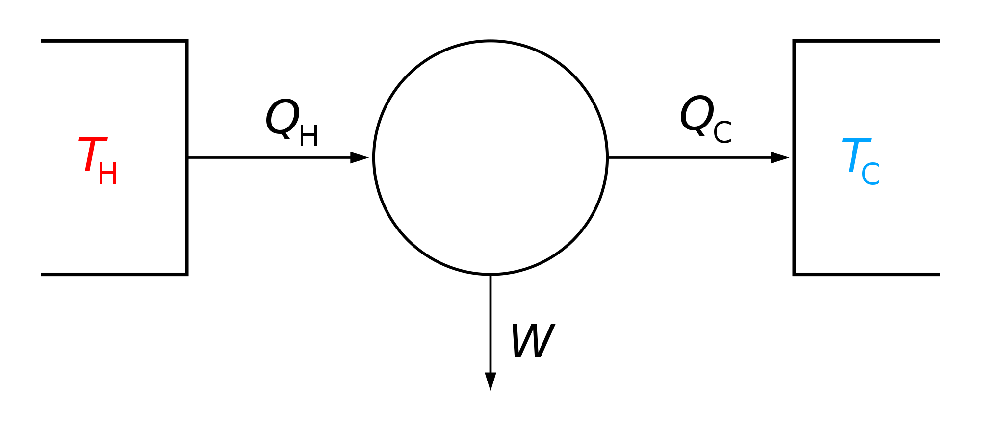
Thermodynamic process
Classical thermodynamics considers three main kinds of thermodynamic processes: (1) changes in a system, (2) cycles in a system, and (3) flow processes.
(1) A Thermodynamic process is a process in which the thermodynamic state of a system is changed. A change in a system is defined by a passage from an initial to a final state of thermodynamic equilibrium. In classical thermodynamics, the actual course of the process is not the primary concern, and often is ignored. A state of thermodynamic equilibrium endures unchangingly unless it is interrupted by a thermodynamic operation that initiates a thermodynamic process. The equilibrium states are each respectively fully specified by a suitable set of thermodynamic state variables, that depend only on the current state of the system, not on the path taken by the processes that produce the state. In general, during the actual course of a thermodynamic process, the system may pass through physical states which are not describable as thermodynamic states, because they are far from internal thermodynamic equilibrium. Non-equilibrium thermodynamics, however, considers processes in which the states of the system are close to thermodynamic equilibrium, and aims to describe the continuous passage along the path, at definite rates of progress.
As a useful theoretical but not actually physically realizable limiting case, a process may be imagined to take place practically infinitely slowly or smoothly enough to allow it to be described by a continuous path of equilibrium thermodynamic states, when it is called a "quasi-static" process. This is a theoretical exercise in differential geometry, as opposed to a description of an actually possible physical process; in this idealized case, the calculation may be exact.
A really possible or actual thermodynamic process, considered closely, involves friction. This contrasts with theoretically idealized, imagined, or limiting, but not actually possible, quasi-static processes which may occur with a theoretical slowness that avoids friction. It also contrasts with idealized frictionless processes in the surroundings, which may be thought of as including 'purely mechanical systems'; this difference comes close to defining a thermodynamic process.
(2) A cyclic process carries the system through a cycle of stages, starting and being completed in some particular state. The descriptions of the staged states of the system are not the primary concern. The primary concern is the sums of matter and energy inputs and outputs to the cycle. Cyclic processes were important conceptual devices in the early days of thermodynamical investigation, while the concept of the thermodynamic state variable was being developed.
(3) Defined by flows through a system, a flow process is a steady state of flows into and out of a vessel with definite wall properties. The internal state of the vessel contents is not the primary concern. The quantities of primary concern describe the states of the inflow and the outflow materials, and, on the side, the transfers of heat, work, and kinetic and potential energies for the vessel. Flow processes are of interest in engineering.
Defined by a cycle of transfers into and out of a system, a cyclic process is described by the quantities transferred in the several stages of the cycle. The descriptions of the staged states of the system may be of little or even no interest. A cycle is a sequence of a small number of thermodynamic processes that indefinitely often, repeatedly returns the system to its original state. For this, the staged states themselves are not necessarily described, because it is the transfers that are of interest. It is reasoned that if the cycle can be repeated indefinitely often, then it can be assumed that the states are recurrently unchanged. The condition of the system during the several staged processes may be of even less interest than is the precise nature of the recurrent states. If, however, the several staged processes are idealized and quasi-static, then the cycle is described by a path through a continuous progression of equilibrium states.
Defined by flows through a system, a flow process is a steady state of flow into and out of a vessel with definite wall properties. The internal state of the vessel contents is not the primary concern. The quantities of primary concern describe the states of the inflow and the outflow materials, and, on the side, the transfers of heat, work, and kinetic and potential energies for the vessel. The states of the inflow and outflow materials consist of their internal states, and of their kinetic and potential energies as whole bodies. Very often, the quantities that describe the internal states of the input and output materials are estimated on the assumption that they are bodies in their own states of internal thermodynamic equilibrium. Because rapid reactions are permitted, the thermodynamic treatment may be approximate, not exact.
Hub AI
Thermodynamic process AI simulator
(@Thermodynamic process_simulator)
Thermodynamic process
Classical thermodynamics considers three main kinds of thermodynamic processes: (1) changes in a system, (2) cycles in a system, and (3) flow processes.
(1) A Thermodynamic process is a process in which the thermodynamic state of a system is changed. A change in a system is defined by a passage from an initial to a final state of thermodynamic equilibrium. In classical thermodynamics, the actual course of the process is not the primary concern, and often is ignored. A state of thermodynamic equilibrium endures unchangingly unless it is interrupted by a thermodynamic operation that initiates a thermodynamic process. The equilibrium states are each respectively fully specified by a suitable set of thermodynamic state variables, that depend only on the current state of the system, not on the path taken by the processes that produce the state. In general, during the actual course of a thermodynamic process, the system may pass through physical states which are not describable as thermodynamic states, because they are far from internal thermodynamic equilibrium. Non-equilibrium thermodynamics, however, considers processes in which the states of the system are close to thermodynamic equilibrium, and aims to describe the continuous passage along the path, at definite rates of progress.
As a useful theoretical but not actually physically realizable limiting case, a process may be imagined to take place practically infinitely slowly or smoothly enough to allow it to be described by a continuous path of equilibrium thermodynamic states, when it is called a "quasi-static" process. This is a theoretical exercise in differential geometry, as opposed to a description of an actually possible physical process; in this idealized case, the calculation may be exact.
A really possible or actual thermodynamic process, considered closely, involves friction. This contrasts with theoretically idealized, imagined, or limiting, but not actually possible, quasi-static processes which may occur with a theoretical slowness that avoids friction. It also contrasts with idealized frictionless processes in the surroundings, which may be thought of as including 'purely mechanical systems'; this difference comes close to defining a thermodynamic process.
(2) A cyclic process carries the system through a cycle of stages, starting and being completed in some particular state. The descriptions of the staged states of the system are not the primary concern. The primary concern is the sums of matter and energy inputs and outputs to the cycle. Cyclic processes were important conceptual devices in the early days of thermodynamical investigation, while the concept of the thermodynamic state variable was being developed.
(3) Defined by flows through a system, a flow process is a steady state of flows into and out of a vessel with definite wall properties. The internal state of the vessel contents is not the primary concern. The quantities of primary concern describe the states of the inflow and the outflow materials, and, on the side, the transfers of heat, work, and kinetic and potential energies for the vessel. Flow processes are of interest in engineering.
Defined by a cycle of transfers into and out of a system, a cyclic process is described by the quantities transferred in the several stages of the cycle. The descriptions of the staged states of the system may be of little or even no interest. A cycle is a sequence of a small number of thermodynamic processes that indefinitely often, repeatedly returns the system to its original state. For this, the staged states themselves are not necessarily described, because it is the transfers that are of interest. It is reasoned that if the cycle can be repeated indefinitely often, then it can be assumed that the states are recurrently unchanged. The condition of the system during the several staged processes may be of even less interest than is the precise nature of the recurrent states. If, however, the several staged processes are idealized and quasi-static, then the cycle is described by a path through a continuous progression of equilibrium states.
Defined by flows through a system, a flow process is a steady state of flow into and out of a vessel with definite wall properties. The internal state of the vessel contents is not the primary concern. The quantities of primary concern describe the states of the inflow and the outflow materials, and, on the side, the transfers of heat, work, and kinetic and potential energies for the vessel. The states of the inflow and outflow materials consist of their internal states, and of their kinetic and potential energies as whole bodies. Very often, the quantities that describe the internal states of the input and output materials are estimated on the assumption that they are bodies in their own states of internal thermodynamic equilibrium. Because rapid reactions are permitted, the thermodynamic treatment may be approximate, not exact.