Uniform continuity

For a function ${\displaystyle f:X\to Y}$ with metric spaces ${\displaystyle (X,d_{1})}$ and ${\displaystyle (Y,d_{2})}$, the following definitions of uniform continuity and (ordinary) continuity hold.

• ${\displaystyle f}$ is called uniformly continuous if for every real number ${\displaystyle \varepsilon >0}$ there exists a real number ${\displaystyle \delta >0}$ such that for every ${\displaystyle x,y\in X}$ with ${\displaystyle d_{1}(x,y)<\delta }$, we have ${\displaystyle d_{2}(f(x),f(y))<\varepsilon }$. The set ${\displaystyle \{y\in X:d_{1}(x,y)<\delta \}}$ for each ${\displaystyle x}$ is a neighbourhood of ${\displaystyle x}$ and the set ${\displaystyle \{x\in X:d_{1}(x,y)<\delta \}}$ for each ${\displaystyle y}$ is a neighbourhood of ${\displaystyle y}$ by the definition of a neighbourhood in a metric space.
  • If ${\displaystyle X}$ and ${\displaystyle Y}$ are subsets of the real line, then ${\displaystyle d_{1}}$ and ${\displaystyle d_{2}}$ can be the standard one-dimensional Euclidean distance, yielding the following definition: for every real number ${\displaystyle \varepsilon >0}$ there exists a real number ${\displaystyle \delta >0}$ such that for every ${\displaystyle x,y\in X}$, ${\displaystyle |x-y|<\delta \implies |f(x)-f(y)|<\varepsilon }$ (where ${\displaystyle A\implies B}$ is a material conditional statement saying "if ${\displaystyle A}$, then ${\displaystyle B}$").
• Equivalently, ${\displaystyle f}$ is said to be uniformly continuous if ${\displaystyle \forall \varepsilon >0\;\exists \delta >0\;\forall x\in X\;\forall y\in X:\,d_{1}(x,y)<\delta \,\Rightarrow \,d_{2}(f(x),f(y))<\varepsilon }$. Here quantifications (${\displaystyle \forall \varepsilon >0}$, ${\displaystyle \exists \delta >0}$, ${\displaystyle \forall x\in X}$, and ${\displaystyle \forall y\in X}$) are used.
• Equivalently, ${\displaystyle f}$ is uniformly continuous if it admits a modulus of continuity.

• ${\displaystyle f}$ is called continuous ${\displaystyle {\underline {{\text{at }}x}}}$ if for every real number ${\displaystyle \varepsilon >0}$ there exists a real number ${\displaystyle \delta >0}$ such that for every ${\displaystyle y\in X}$ with ${\displaystyle d_{1}(x,y)<\delta }$, we have ${\displaystyle d_{2}(f(x),f(y))<\varepsilon }$. The set ${\displaystyle \{y\in X:d_{1}(x,y)<\delta \}}$ is a neighbourhood of ${\displaystyle x}$. Thus, (ordinary) continuity is a local property of the function at the point ${\displaystyle x}$.
• Equivalently, a function ${\displaystyle f}$ is said to be continuous if ${\displaystyle \forall x\in X\;\forall \varepsilon >0\;\exists \delta >0\;\forall y\in X:\,d_{1}(x,y)<\delta \,\Rightarrow \,d_{2}(f(x),f(y))<\varepsilon }$.
• Alternatively, a function ${\displaystyle f}$ is said to be continuous if there is a function of all positive real numbers ${\displaystyle \varepsilon }$ and ${\displaystyle x\in X}$, ${\displaystyle \delta (\varepsilon ,x)}$ representing the maximum positive real number, such that at each ${\displaystyle x}$ if ${\displaystyle y\in X}$ satisfies ${\displaystyle d_{1}(x,y)<\delta (\varepsilon ,x)}$ then ${\displaystyle d_{2}(f(x),f(y))<\varepsilon }$. At every ${\displaystyle x}$, ${\displaystyle \delta (\varepsilon ,x)}$ is a monotonically non-decreasing function.

In the definitions, the difference between uniform continuity and continuity is that, in uniform continuity there is a globally applicable ${\displaystyle \delta }$ (the size of a neighbourhood in ${\displaystyle X}$ over which values of the metric for function values in ${\displaystyle Y}$ are less than ${\displaystyle \varepsilon }$) that depends on only ${\displaystyle \varepsilon }$ while in continuity there is a locally applicable ${\displaystyle \delta }$ that depends on the both ${\displaystyle \varepsilon }$ and ${\displaystyle x}$. Continuity is a local property of a function — that is, a function ${\displaystyle f}$ is continuous, or not, at a particular point ${\displaystyle x}$ of the function domain ${\displaystyle X}$, and this can be determined by looking at only the values of the function in an arbitrarily small neighbourhood of that point. When we speak of a function being continuous on an interval, we mean that the function is continuous at every point of the interval. In contrast, uniform continuity is a global property of ${\displaystyle f}$, in the sense that the standard definition of uniform continuity refers to every point of ${\displaystyle X}$. On the other hand, it is possible to give a definition that is local in terms of the natural extension ${\displaystyle f^{*}}$(the characteristics of which at nonstandard points are determined by the global properties of ${\displaystyle f}$), although it is not possible to give a local definition of uniform continuity for an arbitrary hyperreal-valued function, see below.

A mathematical definition that a function ${\displaystyle f}$ is continuous on an interval ${\displaystyle I}$ and a definition that ${\displaystyle f}$ is uniformly continuous on ${\displaystyle I}$ are structurally similar as shown in the following.

Continuity of a function ${\displaystyle f:X\to Y}$ for metric spaces ${\displaystyle (X,d_{1})}$ and ${\displaystyle (Y,d_{2})}$ at every point ${\displaystyle x}$ of an interval ${\displaystyle I\subseteq X}$ (i.e., continuity of ${\displaystyle f}$ on the interval ${\displaystyle I}$) is expressed by a formula starting with quantifications

${\displaystyle \forall x\in I\;\forall \varepsilon >0\;\exists \delta >0\;\forall y\in I:\,d_{1}(x,y)<\delta \,\Rightarrow \,d_{2}(f(x),f(y))<\varepsilon }$,

(metrics ${\displaystyle d_{1}(x,y)}$ and ${\displaystyle d_{2}(f(x),f(y))}$ are ${\displaystyle |x-y|}$ and ${\displaystyle |f(x)-f(y)|}$ for ${\displaystyle f:\mathbb {R} \to \mathbb {R} }$ for the set of real numbers ${\displaystyle \mathbb {R} }$).

For uniform continuity, the order of the first, second, and third quantifications (${\displaystyle \forall x\in I}$, ${\displaystyle \forall \varepsilon >0}$, and ${\displaystyle \exists \delta >0}$) are rotated:

${\displaystyle \forall \varepsilon >0\;\exists \delta >0\;\forall x\in I\;\forall y\in I:\,d_{1}(x,y)<\delta \,\Rightarrow \,d_{2}(f(x),f(y))<\varepsilon }$.

Thus for continuity on the interval, one takes an arbitrary point ${\displaystyle x}$ of the interval, and then there must exist a distance ${\displaystyle \delta }$,

${\displaystyle \cdots \forall x\,\exists \delta \cdots ,}$

while for uniform continuity, a single ${\displaystyle \delta }$ must work uniformly for all points ${\displaystyle x}$ of the interval,

${\displaystyle \cdots \exists \delta \,\forall x\cdots .}$

Every uniformly continuous function is continuous, but the converse does not hold. Consider for instance the continuous function ${\displaystyle f\colon \mathbb {R} \rightarrow \mathbb {R} ,x\mapsto x^{2}}$ where ${\displaystyle \mathbb {R} }$ is the set of real numbers. Given a positive real number ${\displaystyle \varepsilon }$, uniform continuity requires the existence of a positive real number ${\displaystyle \delta }$ such that for all ${\displaystyle x_{1},x_{2}\in \mathbb {R} }$ with ${\displaystyle |x_{1}-x_{2}|<\delta }$, we have ${\displaystyle |f(x_{1})-f(x_{2})|<\varepsilon }$. But

${\displaystyle f\left(x+\delta \right)-f(x)=2x\cdot \delta +\delta ^{2},}$

and as ${\displaystyle x}$ goes to be a higher and higher value, ${\displaystyle \delta }$ needs to be lower and lower to satisfy ${\displaystyle |f(x+\beta )-f(x)|<\varepsilon }$ for positive real numbers ${\displaystyle \beta <\delta }$ and the given ${\displaystyle \varepsilon }$. This means that there is no specifiable (no matter how small it is) positive real number ${\displaystyle \delta }$ to satisfy the condition for ${\displaystyle f}$ to be uniformly continuous so ${\displaystyle f}$ is not uniformly continuous.

Any absolutely continuous function (over a compact interval) is uniformly continuous. On the other hand, the Cantor function is uniformly continuous but not absolutely continuous.

The image of a totally bounded subset under a uniformly continuous function is totally bounded. However, the image of a bounded subset of an arbitrary metric space under a uniformly continuous function need not be bounded: as a counterexample, consider the identity function from the integers endowed with the discrete metric to the integers endowed with the usual Euclidean metric.

The Heine–Cantor theorem asserts that every continuous function on a compact set is uniformly continuous. In particular, if a function is continuous on a closed bounded interval of the real line, it is uniformly continuous on that interval. The Darboux integrability of continuous functions follows almost immediately from this theorem.

If a real-valued function ${\displaystyle f}$ is continuous on ${\displaystyle [0,\infty )}$ and ${\displaystyle \lim _{x\to \infty }f(x)}$ exists (and is finite), then ${\displaystyle f}$ is uniformly continuous. In particular, every element of ${\displaystyle C_{0}(\mathbb {R} )}$, the space of continuous functions on ${\displaystyle \mathbb {R} }$ that vanish at infinity, is uniformly continuous. This is a generalization of the Heine-Cantor theorem mentioned above, since ${\displaystyle C_{c}(\mathbb {R} )\subset C_{0}(\mathbb {R} )}$.

• Linear functions ${\displaystyle x\mapsto ax+b}$ are the simplest examples of uniformly continuous functions.
• Any continuous function on the interval ${\displaystyle [0,1]}$ is also uniformly continuous, since ${\displaystyle [0,1]}$ is a compact set.
• If a function is differentiable on an open interval and its derivative is bounded, then the function is uniformly continuous on that interval.
• Every Lipschitz continuous map between two metric spaces is uniformly continuous. More generally, every Hölder continuous function is uniformly continuous.
• The absolute value function is uniformly continuous, despite not being differentiable at ${\displaystyle x=0}$. This shows uniformly continuous functions are not always differentiable.
• Despite being nowhere differentiable, the Weierstrass function is uniformly continuous.
• Every member of a uniformly equicontinuous set of functions is uniformly continuous.

• Functions that are unbounded on a bounded domain are not uniformly continuous. The tangent function is continuous on the interval ${\displaystyle (-\pi /2,\pi /2)}$ but is not uniformly continuous on that interval, as it goes to infinity as ${\displaystyle x\to \pi /2}$.
• Functions whose derivative tends to infinity as ${\displaystyle x}$ grows large cannot be uniformly continuous. The exponential function ${\displaystyle x\mapsto e^{x}}$ is continuous everywhere on the real line but is not uniformly continuous on the line, since its derivative is ${\displaystyle e^{x}}$, and ${\displaystyle e^{x}\to \infty }$ as ${\displaystyle x\to \infty }$.

For a uniformly continuous function, for every positive real number ${\displaystyle \varepsilon >0}$ there is a positive real number ${\displaystyle \delta >0}$ such that two function values ${\displaystyle f(x)}$ and ${\displaystyle f(y)}$ have the maximum distance ${\displaystyle \varepsilon }$ whenever ${\displaystyle x}$ and ${\displaystyle y}$ are within the maximum distance ${\displaystyle \delta }$. Thus at each point ${\displaystyle (x,f(x))}$ of the graph, if we draw a rectangle with a height slightly less than ${\displaystyle 2\varepsilon }$ and width a slightly less than ${\displaystyle 2\delta }$ around that point, then the graph lies completely within the height of the rectangle, i.e., the graph do not pass through the top or the bottom side of the rectangle. For functions that are not uniformly continuous, this isn't possible; for these functions, the graph might lie inside the height of the rectangle at some point on the graph but there is a point on the graph where the graph lies above or below the rectangle. (the graph penetrates the top or bottom side of the rectangle.)

• 
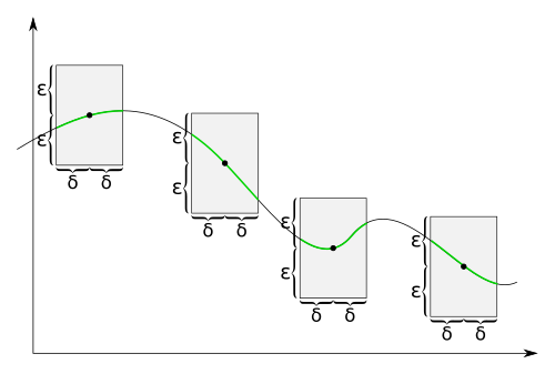  For uniformly continuous functions, for each positive real number ${\displaystyle \varepsilon >0}$ there is a positive real number ${\displaystyle \delta >0}$ such that when we draw a rectangle around each point of the graph with a width slightly less than ${\displaystyle 2\delta }$ and a height slightly less than ${\displaystyle 2\varepsilon }$, the graph lies completely inside the height of the rectangle.
• 
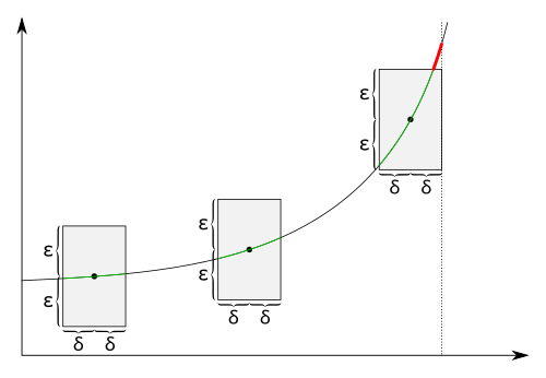  For functions that are not uniformly continuous, there is a positive real number ${\displaystyle \varepsilon >0}$ such that for every positive real number ${\displaystyle \delta >0}$ there is a point on the graph so that when we draw a rectangle with a height slightly less than ${\displaystyle 2\varepsilon }$ and a width slightly less than ${\displaystyle 2\delta }$ around that point, there is a function value directly above or below the rectangle. There might be a graph point where the graph is completely inside the height of the rectangle but this is not true for every point of the graph.

The first published definition of uniform continuity was by Heine in 1870, and in 1872 he published a proof that a continuous function on an open interval need not be uniformly continuous. The proofs are almost verbatim given by Dirichlet in his lectures on definite integrals in 1854. The definition of uniform continuity appears earlier in the work of Bolzano where he also proved that continuous functions on an open interval do not need to be uniformly continuous. In addition he also states that a continuous function on a closed interval is uniformly continuous, but he does not give a complete proof.^[1]

In non-standard analysis, a real-valued function ${\displaystyle f}$ of a real variable is microcontinuous at a point ${\displaystyle a}$ precisely if the difference ${\displaystyle f^{*}(a+\delta )-f^{*}(a)}$ is infinitesimal whenever ${\displaystyle \delta }$ is infinitesimal. Thus ${\displaystyle f}$ is continuous on a set ${\displaystyle A}$ in ${\displaystyle \mathbb {R} }$ precisely if ${\displaystyle f^{*}}$ is microcontinuous at every real point ${\displaystyle a\in A}$. Uniform continuity can be expressed as the condition that (the natural extension of) ${\displaystyle f}$ is microcontinuous not only at real points in ${\displaystyle A}$, but at all points in its non-standard counterpart (natural extension) ${\displaystyle ^{*}A}$ in ${\displaystyle ^{*}\mathbb {R} }$. Note that there exist hyperreal-valued functions which meet this criterion but are not uniformly continuous, as well as uniformly continuous hyperreal-valued functions which do not meet this criterion, however, such functions cannot be expressed in the form ${\displaystyle f^{*}}$ for any real-valued function ${\displaystyle f}$. (see non-standard calculus for more details and examples).

For a function between metric spaces, uniform continuity implies Cauchy continuity (Fitzpatrick 2006). More specifically, let ${\displaystyle A}$ be a subset of ${\displaystyle \mathbb {R} ^{n}}$. If a function ${\displaystyle f:A\to \mathbb {R} ^{n}}$ is uniformly continuous then for every pair of sequences ${\displaystyle x_{n}}$ and ${\displaystyle y_{n}}$ such that

${\displaystyle \lim _{n\to \infty }|x_{n}-y_{n}|=0}$

we have

${\displaystyle \lim _{n\to \infty }|f(x_{n})-f(y_{n})|=0.}$

Let ${\displaystyle X}$ be a metric space, ${\displaystyle S}$ a subset of ${\displaystyle X}$, ${\displaystyle R}$ a complete metric space, and ${\displaystyle f:S\rightarrow R}$ a continuous function. A question to answer: When can ${\displaystyle f}$ be extended to a continuous function on all of ${\displaystyle X}$?

If ${\displaystyle S}$ is closed in ${\displaystyle X}$, the answer is given by the Tietze extension theorem. So it is necessary and sufficient to extend ${\displaystyle f}$ to the closure of ${\displaystyle S}$ in ${\displaystyle X}$: that is, we may assume without loss of generality that ${\displaystyle S}$ is dense in ${\displaystyle X}$, and this has the further pleasant consequence that if the extension exists, it is unique. A sufficient condition for ${\displaystyle f}$ to extend to a continuous function ${\displaystyle f:X\rightarrow R}$ is that it is Cauchy-continuous, i.e., the image under ${\displaystyle f}$ of a Cauchy sequence remains Cauchy. If ${\displaystyle X}$ is complete (and thus the completion of ${\displaystyle S}$), then every continuous function from ${\displaystyle X}$ to a metric space ${\displaystyle Y}$ is Cauchy-continuous. Therefore when ${\displaystyle X}$ is complete, ${\displaystyle f}$ extends to a continuous function ${\displaystyle f:X\rightarrow R}$ if and only if ${\displaystyle f}$ is Cauchy-continuous.

It is easy to see that every uniformly continuous function is Cauchy-continuous and thus extends to ${\displaystyle X}$. The converse does not hold, since the function ${\displaystyle f:R\rightarrow R,x\mapsto x^{2}}$ is, as seen above, not uniformly continuous, but it is continuous and thus Cauchy continuous. In general, for functions defined on unbounded spaces like ${\displaystyle R}$, uniform continuity is a rather strong condition. It is desirable to have a weaker condition from which to deduce extendability.

For example, suppose ${\displaystyle a>1}$ is a real number. At the precalculus level, the function ${\displaystyle f:x\mapsto a^{x}}$ can be given a precise definition only for rational values of ${\displaystyle x}$ (assuming the existence of qth roots of positive real numbers, an application of the Intermediate Value Theorem). One would like to extend ${\displaystyle f}$ to a function defined on all of ${\displaystyle R}$. The identity

${\displaystyle f(x+\delta )-f(x)=a^{x}\left(a^{\delta }-1\right)}$

shows that ${\displaystyle f}$ is not uniformly continuous on the set ${\displaystyle Q}$ of all rational numbers; however for any bounded interval ${\displaystyle I}$ the restriction of ${\displaystyle f}$ to ${\displaystyle Q\cap I}$ is uniformly continuous, hence Cauchy-continuous, hence ${\displaystyle f}$ extends to a continuous function on ${\displaystyle I}$. But since this holds for every ${\displaystyle I}$, there is then a unique extension of ${\displaystyle f}$ to a continuous function on all of ${\displaystyle R}$.

More generally, a continuous function ${\displaystyle f:S\rightarrow R}$ whose restriction to every bounded subset of ${\displaystyle S}$ is uniformly continuous is extendable to ${\displaystyle X}$, and the converse holds if ${\displaystyle X}$ is locally compact.

A typical application of the extendability of a uniformly continuous function is the proof of the inverse Fourier transformation formula. We first prove that the formula is true for test functions, there are densely many of them. We then extend the inverse map to the whole space using the fact that linear map is continuous; thus, uniformly continuous.

In the special case of two topological vector spaces ${\displaystyle V}$ and ${\displaystyle W}$, the notion of uniform continuity of a map ${\displaystyle f:V\to W}$ becomes: for any neighborhood ${\displaystyle B}$ of zero in ${\displaystyle W}$, there exists a neighborhood ${\displaystyle A}$ of zero in ${\displaystyle V}$ such that ${\displaystyle v_{1}-v_{2}\in A}$ implies ${\displaystyle f(v_{1})-f(v_{2})\in B.}$

For linear transformations ${\displaystyle f:V\to W}$, uniform continuity is equivalent to continuity. This fact is frequently used implicitly in functional analysis to extend a linear map off a dense subspace of a Banach space.

Just as the most natural and general setting for continuity is topological spaces, the most natural and general setting for the study of uniform continuity are the uniform spaces. A function ${\displaystyle f:X\to Y}$ between uniform spaces is called uniformly continuous if for every entourage ${\displaystyle V}$ in ${\displaystyle Y}$ there exists an entourage ${\displaystyle U}$ in ${\displaystyle X}$ such that for every ${\displaystyle (x_{1},x_{2})}$ in ${\displaystyle U}$ we have ${\displaystyle (f(x_{1}),f(x_{2}))}$ in ${\displaystyle V}$.

In this setting, it is also true that uniformly continuous maps transform Cauchy sequences into Cauchy sequences.

Each compact Hausdorff space possesses exactly one uniform structure compatible with the topology. A consequence is a generalization of the Heine-Cantor theorem: each continuous function from a compact Hausdorff space to a uniform space is uniformly continuous.

• Contraction mapping – Function reducing distance between all points
• Uniform convergence – Mode of convergence of a function sequence
• Uniform isomorphism – Uniformly continuous homeomorphism

References

[edit]Further reading
[edit]- Bourbaki, Nicolas (1989). General Topology: Chapters 1–4 [Topologie Générale]. Springer. ISBN 0-387-19374-X. Chapter II is a comprehensive reference of uniform spaces.
- Dieudonné, Jean (1960). Foundations of Modern Analysis. Academic Press.
- Fitzpatrick, Patrick (2006). Advanced Calculus. Brooks/Cole. ISBN 0-534-92612-6.
- Kelley, John L. (1955). General topology. Graduate Texts in Mathematics. Springer-Verlag. ISBN 0-387-90125-6.
{{cite book}}: ISBN / Date incompatibility (help) - Kudryavtsev, L.D. (2001) [1994], "Uniform continuity", Encyclopedia of Mathematics, EMS Press
- Rudin, Walter (1976). Principles of Mathematical Analysis. New York: McGraw-Hill. ISBN 978-0-07-054235-8.
- Rusnock, P.; Kerr-Lawson, A. (2005), "Bolzano and uniform continuity", Historia Mathematica, 32 (3): 303–311, doi:10.1016/j.hm.2004.11.003