
Community hub
Recent from talks
Contribute something
Nothing was collected or created yet.
IS–LM model
View on Wikipedia
| Part of a series on |
| Macroeconomics |
|---|
_(cropped).jpg) |
The IS–LM model, or Hicks–Hansen model, is a two-dimensional macroeconomic model which is used as a pedagogical tool in macroeconomic teaching. The IS–LM model shows the relationship between interest rates and output in the short run. The intersection of the "investment–saving" (IS) and "liquidity preference–money supply" (LM) curves illustrates a "general equilibrium" where supposed simultaneous equilibria occur in both the goods and the money markets. The IS–LM model shows the importance of various demand shocks (including the effects of monetary policy and fiscal policy) on output and consequently offers an explanation of changes in national income in the short run when prices are fixed or sticky. Hence, the model can be used as a tool to suggest potential levels for appropriate stabilisation policies. It is also used as a building block for the demand side of the economy in more comprehensive models like the AD–AS model.
The model was developed by John Hicks in 1937 and was later extended by Alvin Hansen as a mathematical representation of Keynesian macroeconomic theory. Between the 1940s and mid-1970s, it was the leading framework of macroeconomic analysis. Today, it is generally accepted as being imperfect and is largely absent from teaching at advanced economic levels and from macroeconomic research, but it is still an important pedagogical introductory tool in most undergraduate macroeconomics textbooks.
As monetary policy since the 1980s and 1990s generally does not try to target money supply as assumed in the original IS–LM model, but instead targets interest rate levels directly, some modern versions of the model have changed the interpretation (and in some cases even the name) of the LM curve, presenting it instead simply as a horizontal line showing the central bank's choice of interest rate. This allows for a simpler dynamic adjustment and supposedly reflects the behaviour of actual contemporary central banks more closely.
History
[edit]The IS–LM model was introduced at a conference of the Econometric Society held in Oxford during September 1936. Roy Harrod, John R. Hicks, and James Meade all presented papers describing mathematical models attempting to summarize John Maynard Keynes' General Theory of Employment, Interest, and Money.[1][2] Hicks, who had seen a draft of Harrod's paper, invented the IS–LM model (originally using the abbreviation "LL", not "LM"). He later presented it in "Mr. Keynes and the Classics: A Suggested Interpretation".[1] Hicks and Alvin Hansen developed the model further in the 1930s and early 1940s,[3]: 527 Hansen extending the earlier contribution.[4] The model became a central tool of macroeconomic teaching for many decades. Between the 1940s and mid-1970s, it was the leading framework of macroeconomic analysis.[5] It was particularly suited to illustrate the debate of the 1960s and 1970s between Keynesians and monetarists as to whether fiscal or monetary policy was most effective to stabilize the economy. Later, this issue faded from focus and came to play only a modest role in discussions of short-run fluctuations.[6]
The IS-LM model assumes a fixed price level and consequently cannot in itself be used to analyze inflation. This was of little importance in the 1950s and early 1960s when inflation was not an important issue, but became problematic with the rising inflation levels in the late 1960s and 1970s, which led to extensions of the model to also incorporate aggregate supply in some form, e.g. in the form of the AD–AS model, which can be regarded as an IS-LM model with an added supply side explaining rises in the price level.[6]
One of the basic assumptions of the IS-LM model is that the central bank targets the money supply.[6] However, a fundamental rethinking in central bank policy took place from the early 1990s when central banks generally changed strategies towards targeting inflation rather than money growth and using an interest rate rule to achieve their goal.[3]: 507 As central banks started paying little attention to the money supply when deciding on their policy, this model feature became increasingly unrealistic and sometimes confusing to students.[6] David Romer in 2000 suggested replacing the traditional IS-LM framework with an IS-MP model, replacing the positively sloped LM curve with a horizontal MP curve (where MP stands for "monetary policy"). He advocated that it had several advantages compared to the traditional IS-LM model.[6] John B. Taylor independently made a similar recommendation in the same year.[7] After 2000, this has led to various modifications to the model in many textbooks, replacing the traditional LM curve and story of the central bank influencing the interest rate level indirectly via controlling the supply of money in the money market to a more realistic one of the central bank determining the policy interest rate as an exogenous variable directly.[3]: 113 [8][9]
Today, the IS-LM model is largely absent from macroeconomic research, but it is still a backbone conceptual introductory tool in many macroeconomics textbooks.[10][11]
Formation
[edit]The point where the IS and LM schedules intersect represents a short-run equilibrium in the real and monetary sectors (though not necessarily in other sectors, such as labor markets): both the product market and the money market are in equilibrium.[12] This equilibrium yields a unique combination of the interest rate and real GDP.
IS (investment–saving) curve
[edit]
The IS curve shows the causation from interest rates to planned investment to national income and output.
For the investment–saving curve, the independent variable is the interest rate and the dependent variable is the level of income. The IS curve is drawn as downward-sloping with the interest rate r on the vertical axis and GDP (gross domestic product: Y) on the horizontal axis. The IS curve represents the locus where total spending (consumer spending + planned private investment + government purchases + net exports) equals total output (real income, Y, or GDP).
The IS curve also represents the equilibria where total private investment equals total saving, with saving equal to consumer saving plus government saving (the budget surplus) plus foreign saving (the trade surplus). The level of real GDP (Y) is determined along this line for each interest rate. Every level of the real interest rate will generate a certain level of investment and spending: lower interest rates encourage higher investment and more spending. The multiplier effect of an increase in fixed investment resulting from a lower interest rate raises real GDP. This explains the downward slope of the IS curve. In summary, the IS curve shows the causation from interest rates to planned fixed investment to rising national income and output.
The IS curve is defined by the equation

where Y represents income, represents consumer spending increasing as a function of disposable income (income, Y, minus taxes, T(Y), which themselves depend positively on income), represents business investment decreasing as a function of the real interest rate, G represents government spending, and NX(Y) represents net exports (exports minus imports) decreasing as a function of income (decreasing because imports are an increasing function of income).


LM (liquidity-money) curve
[edit]
The LM curve shows the combinations of interest rates and levels of real income for which the money market is in equilibrium. It shows where money demand equals money supply. For the LM curve, the independent variable is income and the dependent variable is the interest rate.
In the money market equilibrium diagram, the liquidity preference function is the willingness to hold cash. The liquidity preference function is downward sloping (i.e. the willingness to hold cash increases as the interest rate decreases). Two basic elements determine the quantity of cash balances demanded:
- Transactions demand for money: this includes both (a) the willingness to hold cash for everyday transactions and (b) a precautionary measure (money demand in case of emergencies). Transactions demand is positively related to real GDP. As GDP is considered exogenous to the liquidity preference function, changes in GDP shift the curve.
- Speculative demand for money: this is the willingness to hold cash instead of securities as an asset for investment purposes. Speculative demand is inversely related to the interest rate. As the interest rate rises, the opportunity cost of holding money rather than investing in securities increases. So, as interest rates rise, speculative demand for money falls.
Money supply is determined by central bank decisions and willingness of commercial banks to loan money. Money supply in effect is perfectly inelastic with respect to nominal interest rates. Thus the money supply function is represented as a vertical line – money supply is a constant, independent of the interest rate, GDP, and other factors. Mathematically, the LM curve is defined by the equation , where the supply of money is represented as the real amount M/P (as opposed to the nominal amount M), with P representing the price level, and L being the real demand for money, which is some function of the interest rate and the level of real income.

An increase in GDP shifts the liquidity preference function rightward and hence increases the interest rate. Thus the LM function is positively sloped.
Shifts
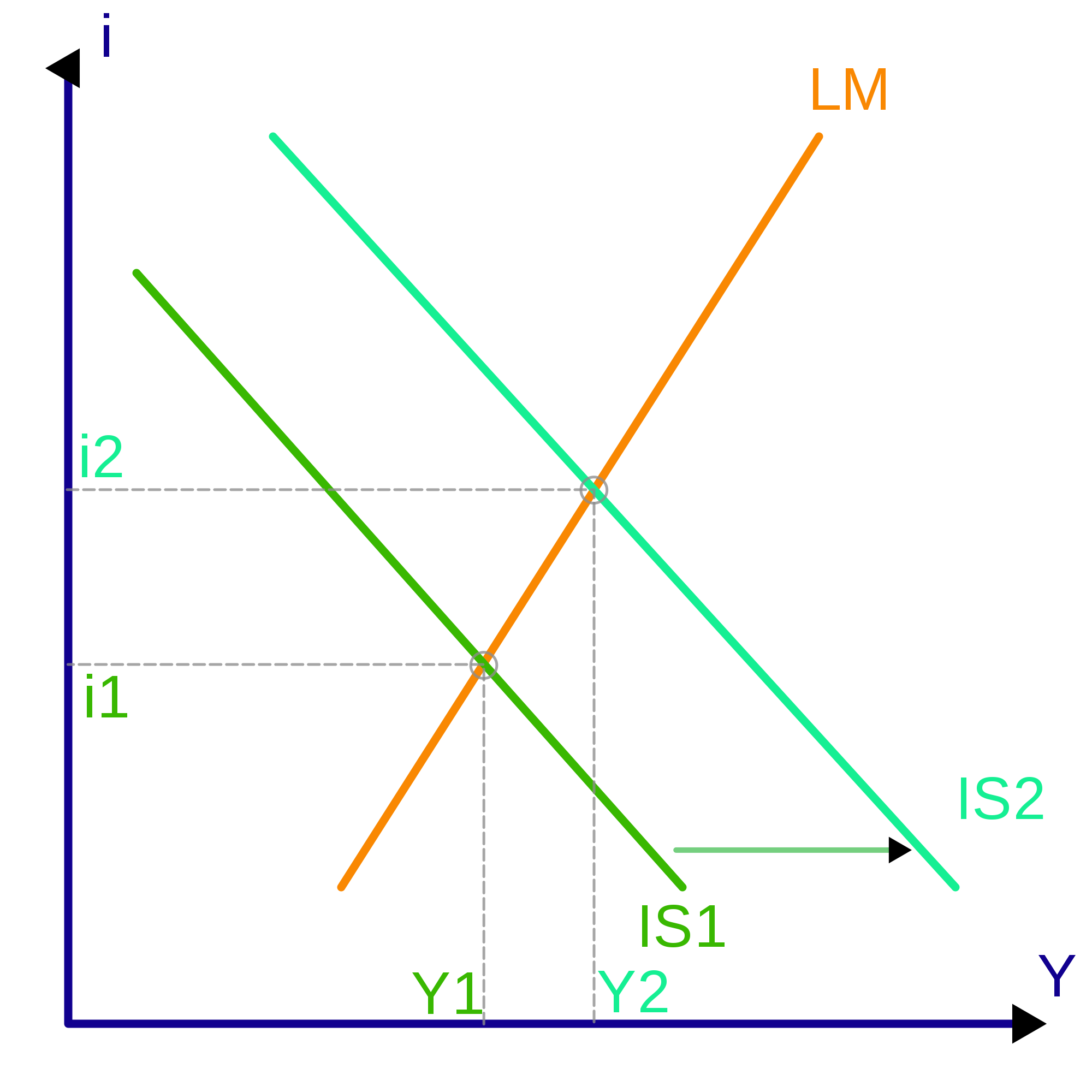
[edit]One hypothesis is that a government's deficit spending ("fiscal policy") has an effect similar to that of a lower saving rate or increased private fixed investment, increasing the amount of demand for goods at each individual interest rate. An increased deficit by the national government shifts the IS curve to the right. This raises the equilibrium interest rate (from i1 to i2) and national income (from Y1 to Y2), as shown in the graph above. The equilibrium level of national income in the IS–LM diagram is referred to as aggregate demand.
Keynesians argue spending may actually "crowd in" (encourage) private fixed investment via the accelerator effect, which helps long-term growth. Further, if government deficits are spent on productive public investment (e.g., infrastructure or public health) that spending directly and eventually raises potential output, although not necessarily more (or less) than the lost private investment might have. The extent of any crowding out depends on the shape of the LM curve. A shift in the IS curve along a relatively flat LM curve can increase output substantially with little change in the interest rate. On the other hand, a rightward shift in the IS curve along a vertical LM curve will lead to higher interest rates, but no change in output (this case represents the "Treasury view").
Rightward shifts of the IS curve also result from exogenous increases in investment spending (i.e., for reasons other than interest rates or income), in consumer spending, and in export spending by people outside the economy being modelled, as well as by exogenous decreases in spending on imports. Thus these too raise both equilibrium income and the equilibrium interest rate. Of course, changes in these variables in the opposite direction shift the IS curve in the opposite direction.
The IS–LM model also allows for the role of monetary policy. If the money supply is increased, that shifts the LM curve downward or to the right, lowering interest rates and raising equilibrium national income. Further, exogenous decreases in liquidity preference, perhaps due to improved transactions technologies, lead to downward shifts of the LM curve and thus increases in income and decreases in interest rates. Changes in these variables in the opposite direction shift the LM curve in the opposite direction.
IS–LM model with interest targeting central bank
[edit]The fact that contemporary central banks normally do not target the money supply, as assumed by the original IS–LM model, but instead conduct their monetary policy by steering the interest rate directly, has led to increasing criticism of the traditional IS–LM setup since 2000 for being outdated and confusing to students. In some textbooks, the traditional LM curve derived from an explicit money market equilibrium story consequently has been replaced by an LM curve simply showing the interest rate level determined by the central bank. Notably this is the case in Olivier Blanchard's widely-used[13] intermediate-level textbook "Macroeconomics" since its 7th edition in 2017.[14]
In this case, the LM curve becomes horizontal at the interest rate level chosen by the central bank, allowing a simpler kind of dynamics. Also, the interest rate level measured along the vertical axis may be interpreted as either the nominal or the real interest rate, in the latter case allowing inflation to enter the IS–LM model in a simple way. The output level is still determined by the intersection of the IS and LM curves. The LM curve may shift because of a change in monetary policy or possibly a change in inflation expectations, whereas the IS curve as in the traditional model may shift either because of a change in fiscal policy affecting government consumption or taxation, or because of shocks affecting private consumption or investment (or, in the open-economy version, net exports). Additionally, the model distinguishes between the policy interest rate determined by the central bank and the market interest rate which is decisive for firms' investment decisions, and which is equal to the policy interest rate plus a premium which may be interpreted as a risk premium or a measure of the market power or other factors influencing the business strategies of commercial banks. This premium allows for shocks in the financial sector being transmitted to the goods market and consequently affecting aggregate demand.[3]: 195–201
Similar models, though called slightly different names, appear in the textbooks by Charles Jones[15] and by Wendy Carlin and David Soskice[14] and the CORE Econ project.[14] Parallelly, texts by Akira Weerapana and Stephen Williamson have outlined approaches where the LM curve is replaced with a real interest rate rule.[15][16]
Incorporation into larger models
[edit]By itself, the traditional IS–LM model is used to study the short run when prices are fixed or sticky, and no inflation is taken into consideration. In addition, the model is often used as a sub-model of larger models which allow for a flexible price level. The addition of a supply relation enables the model to be used for both short- and medium-run analysis of the economy, or to use a different terminology: classical and Keynesian analysis.[15]
A main example of this is the Aggregate Demand-Aggregate Supply model – the AD–AS model.[15] In the aggregate demand-aggregate supply model, each point on the aggregate demand curve is an outcome of the IS–LM model for aggregate demand Y based on a particular price level. Starting from one point on the aggregate demand curve, at a particular price level and a quantity of aggregate demand implied by the IS–LM model for that price level, if one considers a higher potential price level, in the IS–LM model the real money supply M/P will be lower and hence the LM curve will be shifted higher, leading to lower aggregate demand as measured by the horizontal location of the IS–LM intersection; hence at the higher price level the level of aggregate demand is lower, so the aggregate demand curve is negatively sloped.[17]: 315–317
In the 2018 textbook "Macroeconomics" by Daron Acemoglu, David Laibson and John A. List, the corresponding model combining a traditional IS-LM setup with a relation for a changing price level is named an IS-LM-FE model (FE standing for "full equilibrium").[18]
AD-AS-like models with inflation instead of price levels
[edit]In many modern textbooks, the traditional AD–AS diagram is replaced by a variation in which the variables are not output and the price level, but instead output and inflation (i.e., the change in the price level). In this case, the relation corresponding to the AS curve is normally derived from a Phillips curve relationship between inflation and the unemployment gap. As policymakers and economists are generally concerned about inflation levels and not actual price levels, this formulation is considered more appropriate. This variation is often referred to as a dynamic AD–AS model,[9][17] but may also have other names. Olivier Blanchard in his textbook uses the term IS–LM–PC model (PC standing for Phillips curve).[3] Others, among them Carlin and Soskice, refer to it as the "three-equation New Keynesian model",[14] the three equations being an IS relation, often augmented with a term that allows for expectations influencing demand, a monetary policy (interest) rule and a short-run Phillips curve.[15]
Variations
[edit]IS-LM-NAC model
[edit]In 2016, Roger Farmer and Konstantin Platonov presented a so-called IS-LM-NAC model (NAC standing for "no arbitrage condition", in casu between physical capital and financial assets), in which the long-run effect of monetary policy depends on the way in which people form beliefs. The model was an attempt to integrate the phenomenon of secular stagnation in the IS-LM model. Whereas in the IS-LM model, high unemployment would be a temporary phenomenon caused by sticky wages and prices, in the IS-LM-NAC model high unemployment may be a permanent situation caused by pessimistic beliefs - a particular instance of what Keynes called animal spirits.[19] The model was part of a broader research agenda studying how beliefs may independently influence macroeconomic outcomes.[20]
See also
[edit]References
[edit]- ^ a b Hicks, J. R. (1937). "Mr. Keynes and the 'Classics': A Suggested Interpretation". Econometrica. 5 (2): 147–159. doi:10.2307/1907242. JSTOR 1907242.
- ^ Meade, J. E. (1937). "A Simplified Model of Mr. Keynes' System". Review of Economic Studies. 4 (2): 98–107. doi:10.2307/2967607. JSTOR 2967607.
- ^ a b c d e Blanchard, Olivier (2021). Macroeconomics (Eighth, global ed.). Harlow, England: Pearson. ISBN 978-0-134-89789-9.
- ^ Hansen, A. H. (1953). A Guide to Keynes. New York: McGraw Hill. ISBN 9780070260467.
{{cite book}}: ISBN / Date incompatibility (help) - ^ Bentolila, Samuel (2005). "Hicks–Hansen model". An Eponymous Dictionary of Economics: A Guide to Laws and Theorems Named after Economists. Edward Elgar. ISBN 978-1-84376-029-0.
- ^ a b c d e Romer, David (1 May 2000). "Keynesian Macroeconomics without the LM Curve". Journal of Economic Perspectives. 14 (2): 149–170. doi:10.1257/jep.14.2.149. ISSN 0895-3309. Retrieved 9 November 2023.
- ^ Taylor, John B. (May 2000). "Teaching Modern Macroeconomics at the Principles Level". American Economic Review. 90 (2): 90–94. doi:10.1257/aer.90.2.90. ISSN 0002-8282. Retrieved 18 November 2023.
- ^ Romer, David (2019). Advanced macroeconomics (Fifth ed.). New York, NY: McGraw-Hill. p. 262-264. ISBN 978-1-260-18521-8.
- ^ a b Sørensen, Peter Birch; Whitta-Jacobsen, Hans Jørgen (2022). Introducing advanced macroeconomics: growth and business cycles (Third ed.). Oxford, United Kingdom New York, NY: Oxford University Press. p. 606. ISBN 978-0-19-885049-6.
- ^ Colander, David (2004). "The Strange Persistence of the IS-LM Model" (PDF). History of Political Economy. 36 (Annual Supplement): 305–322. CiteSeerX 10.1.1.692.6446. doi:10.1215/00182702-36-suppl_1-305. S2CID 6705939.
- ^ Mankiw, N. Gregory (May 2006). "The Macroeconomist as Scientist and Engineer" (PDF). p. 19. Retrieved 2014-11-17.
- ^ Gordon, Robert J. (2009). Macroeconomics (Eleventh ed.). Boston: Pearson Addison Wesley. ISBN 9780321552075.
- ^ Courtoy, François; De Vroey, Michel; Turati, Riccardo. "What do we teach in Macroeconomics? Evidence of a Theoretical Divide" (PDF). sites.uclouvain.be. UCLouvain. Retrieved 17 November 2023.
- ^ a b c d Davis, Leila E.; Gómez-Ramírez, Leopoldo (2 October 2022). "Teaching post-intermediate macroeconomics with a dynamic 3-equation model". The Journal of Economic Education. 53 (4): 348–367. doi:10.1080/00220485.2022.2111385. ISSN 0022-0485. S2CID 252249958. Retrieved 17 November 2023.
- ^ a b c d e de Araujo, Pedro; O’Sullivan, Roisin; Simpson, Nicole B. (January 2013). "What Should be Taught in Intermediate Macroeconomics?". The Journal of Economic Education. 44 (1): 74–90. doi:10.1080/00220485.2013.740399. ISSN 0022-0485. S2CID 17167083. Retrieved 17 November 2023.
- ^ Weerapana, Akila (2003). "Intermediate Macroeconomics without the IS-LM Model". The Journal of Economic Education. 34 (3): 241–262. doi:10.1080/00220480309595219. ISSN 0022-0485. JSTOR 30042548. S2CID 144412209. Retrieved 18 November 2023.
- ^ a b Mankiw, Nicholas Gregory (2022). Macroeconomics (Eleventh, international ed.). New York, NY: Worth Publishers, Macmillan Learning. ISBN 978-1-319-26390-4.
- ^ Acemoglu, Daron; David I. Laibson; John A. List (2018). Macroeconomics (Second ed.). New York: Pearson. ISBN 978-0-13-449205-6. OCLC 956396690.
- ^ Farmer, Roger E. A. (2016-09-02). "Reinventing IS-LM: The IS-LM-NAC model and how to use it". Vox EU. Retrieved 2020-10-01.
- ^ Farmer, Roger E. A.; Platonov, Konstantin (2019). "Animal spirits in a monetary model" (PDF). European Economic Review. 115: 60–77. doi:10.1016/j.euroecorev.2019.02.005. S2CID 55928575.
Further reading
[edit]- Barro, Robert J. (1984). "The Keynesian Theory of Business Fluctuations". Macroeconomics. New York: John Wiley. pp. 487–513. ISBN 978-0-471-87407-2.
- Blanchard, Olivier (2021). "Goods and Financial Markets: The IS-LM Model". Macroeconomics (Eighth, global ed.). Harlow, England: Pearson. pp. 107–126. ISBN 978-0-134-89789-9.
- Hicks, J. R. (1937). "Mr. Keynes and the 'Classics': A Suggested Interpretation". Econometrica. 5 (2): 147–159. doi:10.2307/1907242. JSTOR 1907242.
- Krugman, Paul (2011-10-09). "IS-LMentary". The New York Times. Retrieved 2020-10-01.
- Leijonhufvud, Axel (1983). "What is Wrong with IS/LM?". In Fitoussi, Jean-Paul (ed.). Modern Macroeconomic Theory. Oxford: Blackwell. pp. 49–90. ISBN 978-0-631-13158-8.
- Mankiw, Nicholas Gregory (2022). "Aggregate Demand I+II". Macroeconomics (Eleventh, international ed.). New York, NY: Worth Publishers, Macmillan Learning. pp. 283–334. ISBN 978-1-319-26390-4.
- Romer, David (2000). "Keynesian Macroeconomics without the LM Curve". Journal of Economic Perspectives. 14 (2): 149–170. doi:10.1257/jep.14.2.149. ISSN 0895-3309.
- Smith, Warren L. (1956). "A Graphical Exposition of the Complete Keynesian System". Southern Economic Journal. 23 (2): 115–125. doi:10.2307/1053551. JSTOR 1053551.
- Vroey, Michel de; Hoover, Kevin D., eds. (2004). The IS-LM model: Its Rise, Fall, and Strange Persistence. Durham: Duke University Press. ISBN 978-0-8223-6631-7.
- Young, Warren; Zilberfarb, Ben-Zion, eds. (2000). IS-LM and Modern Macroeconomics. Recent Economic Thought. Vol. 73. Springer Science & Business Media. doi:10.1007/978-94-010-0644-6. ISBN 978-0-7923-7966-9.
External links
[edit]- Krugman, Paul. There's something about macro – An explanation of the model and its role in understanding macroeconomics.
- Krugman, Paul. IS-LMentary – A basic explanation of the model and its uses.
- Wiens, Elmer G. IS–LM model – An online, interactive IS–LM model of the Canadian economy.
| National | |
|---|---|
| Other | |