In the ordinary least squares solution of

${\displaystyle \mathbf {y} =\mathbf {X} {\boldsymbol {\beta }}+{\boldsymbol {\varepsilon }},\,}$

the problem of a near-singular moment matrix ${\displaystyle \mathbf {X} ^{\mathsf {T}}\mathbf {X} }$ is alleviated by adding positive elements to the diagonals, thereby decreasing its condition number. Compared to the ordinary least squares estimator, the simple ridge estimator has an extra term ${\displaystyle \lambda \mathbf {I} }$ in the denominator: $${\displaystyle {\hat {\boldsymbol {\beta }}}_{R}=\left(\mathbf {X} ^{\mathsf {T}}\mathbf {X} +\lambda \mathbf {I} \right)^{-1}\mathbf {X} ^{\mathsf {T}}\mathbf {y} }$$ where ${\displaystyle \mathbf {y} }$ is the regressand, ${\displaystyle \mathbf {X} }$ is the design matrix, ${\displaystyle \mathbf {I} }$ is the identity matrix, and the ridge parameter ${\displaystyle \lambda \geq 0}$ serves as the constant shifting the diagonals of the moment matrix.^[8] It can be shown that this estimator is the solution to the least squares problem subject to the constraint ${\displaystyle {\boldsymbol {\beta }}^{\mathsf {T}}{\boldsymbol {\beta }}=c}$, which can be expressed as a Lagrangian minimization: $${\displaystyle {\hat {\boldsymbol {\beta }}}_{R}={\text{argmin}}_{\boldsymbol {\beta }}\,\left(\mathbf {y} -\mathbf {X} {\boldsymbol {\beta }}\right)^{\mathsf {T}}\left(\mathbf {y} -\mathbf {X} {\boldsymbol {\beta }}\right)+\lambda \left({\boldsymbol {\beta }}^{\mathsf {T}}{\boldsymbol {\beta }}-c\right)}$$ which shows that ${\displaystyle \lambda }$ is nothing but the Lagrange multiplier of the constraint.^[9] In fact, there is a one-to-one relationship between ${\displaystyle c}$ and ${\displaystyle \beta }$ and since, in practice, we do not know ${\displaystyle c}$, we define ${\displaystyle \lambda }$ heuristically or find it via additional data-fitting strategies, see Determination of the Tikhonov factor.

Note that, when ${\displaystyle \lambda =0}$, in which case the constraint is non-binding, the ridge estimator reduces to ordinary least squares. A more general approach to Tikhonov regularization is discussed below.

Tikhonov regularization was invented independently in many different contexts. It became widely known through its application to integral equations in the works of Andrey Tikhonov^{[10][11][12][13][14]} and David L. Phillips.^[15] Some authors use the term Tikhonov–Phillips regularization. The finite-dimensional case was expounded by Arthur E. Hoerl, who took a statistical approach,^[16] and by Manus Foster, who interpreted this method as a Wiener–Kolmogorov (Kriging) filter.^[17] Following Hoerl, it is known in the statistical literature as ridge regression,^[18] named after ridge analysis ("ridge" refers to the path from the constrained maximum).^[19]

Suppose that for a known real matrix ${\displaystyle A}$ and vector ${\displaystyle \mathbf {b} }$, we wish to find a vector ${\displaystyle \mathbf {x} }$ such that $${\displaystyle A\mathbf {x} =\mathbf {b} ,}$$ where ${\displaystyle \mathbf {x} }$ and ${\displaystyle \mathbf {b} }$ may be of different sizes and ${\displaystyle A}$ may be non-square.

The standard approach is ordinary least squares linear regression.^{[clarification needed]} However, if no ${\displaystyle \mathbf {x} }$ satisfies the equation or more than one ${\displaystyle \mathbf {x} }$ does—that is, the solution is not unique—the problem is said to be ill posed. In such cases, ordinary least squares estimation leads to an overdetermined, or more often an underdetermined system of equations. Most real-world phenomena have the effect of low-pass filters^{[clarification needed]} in the forward direction where ${\displaystyle A}$ maps ${\displaystyle \mathbf {x} }$ to ${\displaystyle \mathbf {b} }$. Therefore, in solving the inverse-problem, the inverse mapping operates as a high-pass filter that has the undesirable tendency of amplifying noise (eigenvalues / singular values are largest in the reverse mapping where they were smallest in the forward mapping). In addition, ordinary least squares implicitly nullifies every element of the reconstructed version of ${\displaystyle \mathbf {x} }$ that is in the null-space of ${\displaystyle A}$, rather than allowing for a model to be used as a prior for ${\displaystyle \mathbf {x} }$. Ordinary least squares seeks to minimize the sum of squared residuals, which can be compactly written as $${\displaystyle \left\|A\mathbf {x} -\mathbf {b} \right\|_{2}^{2},}$$ where ${\displaystyle \|\cdot \|_{2}}$ is the Euclidean norm.

In order to give preference to a particular solution with desirable properties, a regularization term can be included in this minimization: $${\displaystyle \left\|A\mathbf {x} -\mathbf {b} \right\|_{2}^{2}+\left\|\Gamma \mathbf {x} \right\|_{2}^{2}=\left\|{\mathcal {A}}\mathbf {x} -{\mathcal {b}}\right\|_{2}^{2},}$$ where ${\displaystyle {\mathcal {A}}={\begin{pmatrix}A\\\Gamma \end{pmatrix}}}$ and ${\displaystyle {\mathcal {b}}={\begin{pmatrix}\mathbf {b} \\{\boldsymbol {0}}\end{pmatrix}}}$, for some suitably chosen Tikhonov matrix ${\displaystyle \Gamma }$. In many cases, this matrix is chosen as a scalar multiple of the identity matrix (${\displaystyle \Gamma =\alpha I}$), giving preference to solutions with smaller norms; this is known as L₂ regularization.^[20] In other cases, high-pass operators (e.g., a difference operator or a weighted Fourier operator) may be used to enforce smoothness if the underlying vector is believed to be mostly continuous. This regularization improves the conditioning of the problem, thus enabling a direct numerical solution. Treating it as an ordinary least squares problem with augmented matrices ${\displaystyle {\mathcal {A}}}$ and ${\displaystyle {\mathcal {b}}}$, the solution is $${\displaystyle {\hat {\mathbf {x} }}=({\mathcal {A}}^{\mathsf {T}}{\mathcal {A}})^{-1}{\mathcal {A}}^{\mathsf {T}}\mathbf {\mathcal {b}} =(A^{\mathsf {T}}A+\Gamma ^{\mathsf {T}}\Gamma )^{-1}A^{\mathsf {T}}\mathbf {b} .}$$ The effect of regularization may be varied by the scale of the matrix ${\displaystyle \Gamma }$. For ${\displaystyle \Gamma =0}$ this reduces to the unregularized least-squares solution, provided that (A^TA)⁻¹ exists. Note that in case of a complex matrix ${\displaystyle A}$, as usual the transpose ${\displaystyle A^{\mathsf {T}}}$ has to be replaced by the Hermitian transpose ${\displaystyle A^{\mathsf {H}}}$.

L₂ regularization is used in many contexts aside from linear regression, such as classification with logistic regression or support vector machines,^[21] and matrix factorization.^[22]

Since Tikhonov Regularization simply adds a quadratic term to the objective function in optimization problems, it is possible to do so after the unregularised optimisation has taken place. E.g., if the above problem with ${\displaystyle \Gamma =0}$ yields the solution ${\displaystyle {\hat {\mathbf {x} }}_{0}}$, the solution in the presence of ${\displaystyle \Gamma \neq 0}$ can be expressed as: $${\displaystyle {\hat {\mathbf {x} }}=B{\hat {\mathbf {x} }}_{0},}$$ with the "regularisation matrix" ${\displaystyle B=\left(A^{\mathsf {T}}A+\Gamma ^{\mathsf {T}}\Gamma \right)^{-1}A^{\mathsf {T}}A}$.

If the parameter fit comes with a covariance matrix of the estimated parameter uncertainties ${\displaystyle V_{0}}$, then the regularisation matrix will be $${\displaystyle B=(V_{0}^{-1}+\Gamma ^{\mathsf {T}}\Gamma )^{-1}V_{0}^{-1},}$$ and the regularised result will have a new covariance $${\displaystyle V=BV_{0}B^{\mathsf {T}}.}$$

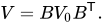
In the context of arbitrary likelihood fits, this is valid, as long as the quadratic approximation of the likelihood function is valid. This means that, as long as the perturbation from the unregularised result is small, one can regularise any result that is presented as a best fit point with a covariance matrix. No detailed knowledge of the underlying likelihood function is needed.^[23]

For general multivariate normal distributions for ${\displaystyle \mathbf {x} }$ and the data error, one can apply a transformation of the variables to reduce to the case above. Equivalently, one can seek an ${\displaystyle \mathbf {x} }$ to minimize $${\displaystyle \left\|A\mathbf {x} -\mathbf {b} \right\|_{P}^{2}+\left\|\mathbf {x} -\mathbf {x} _{0}\right\|_{Q}^{2},}$$ where we have used ${\displaystyle \left\|\mathbf {x} \right\|_{Q}^{2}}$ to stand for the weighted norm squared ${\displaystyle \mathbf {x} ^{\mathsf {T}}Q\mathbf {x} }$ (compare with the Mahalanobis distance). In the Bayesian interpretation ${\displaystyle P}$ is the inverse covariance matrix of ${\displaystyle \mathbf {b} }$, ${\displaystyle \mathbf {x} _{0}}$ is the expected value of ${\displaystyle \mathbf {x} }$, and ${\displaystyle Q}$ is the inverse covariance matrix of ${\displaystyle \mathbf {x} }$.

The Tikhonov matrix is not explicitly included because the corresponding regularization term ${\displaystyle \left\|\Gamma \mathbf {x} -\mathbf {x} _{0}'\right\|_{Q'}^{2}}$ reduces to above with ${\displaystyle \Gamma \mathbf {x} _{0}=\mathbf {x} _{0}'}$ and ${\displaystyle Q=\Gamma ^{T}Q'\Gamma }$. For normal regularization where ${\displaystyle Q'=I}$, the Tikhonov matrix then appears in the Cholesky factorization ${\displaystyle Q=\Gamma ^{\mathsf {T}}\Gamma }$ and is considered a whitening filter.

This generalized problem has an optimal solution ${\displaystyle {\hat {\mathbf {x} }}}$ which can be written explicitly using the formula $${\displaystyle \mathbf {\hat {\mathbf {x} }} =\left(A^{\mathsf {T}}PA+Q\right)^{-1}\left(A^{\mathsf {T}}P\mathbf {b} +Q\mathbf {x} _{0}\right)=\mathbf {x} _{0}+\left(A^{\mathsf {T}}PA+Q\right)^{-1}\left(A^{\mathsf {T}}P\left(\mathbf {b} -A\mathbf {x} _{0}\right)\right).}$$

In some situations, one can avoid using the transpose ${\displaystyle A^{\mathsf {T}}}$, as proposed by Mikhail Lavrentyev.^[24] For example, if ${\displaystyle A}$ is symmetric positive definite, i.e. ${\displaystyle A=A^{\mathsf {T}}>0}$, so is its inverse ${\displaystyle A^{-1}}$, which can thus be used to set up the weighted norm squared ${\displaystyle \left\|\mathbf {x} \right\|_{P}^{2}=\mathbf {x} ^{\mathsf {T}}A^{-1}\mathbf {x} }$ in the generalized Tikhonov regularization, leading to minimizing $${\displaystyle \left\|A\mathbf {x} -\mathbf {b} \right\|_{A^{-1}}^{2}+\left\|\mathbf {x} -\mathbf {x} _{0}\right\|_{Q}^{2}}$$ or, equivalently up to a constant term, $${\displaystyle \mathbf {x} ^{\mathsf {T}}\left(A+Q\right)\mathbf {x} -2\mathbf {x} ^{\mathsf {T}}\left(\mathbf {b} +Q\mathbf {x} _{0}\right).}$$

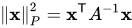
This minimization problem has an optimal solution ${\displaystyle \mathbf {x} ^{*}}$ which can be written explicitly using the formula $${\displaystyle \mathbf {x} ^{*}=\left(A+Q\right)^{-1}\left(\mathbf {b} +Q\mathbf {x} _{0}\right),}$$ which is nothing but the solution of the generalized Tikhonov problem where ${\displaystyle A=A^{\mathsf {T}}=P^{-1}.}$

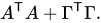
The Lavrentyev regularization, if applicable, is advantageous to the original Tikhonov regularization, since the Lavrentyev matrix ${\displaystyle A+Q}$ can be better conditioned, i.e., have a smaller condition number, compared to the Tikhonov matrix ${\displaystyle A^{\mathsf {T}}A+\Gamma ^{\mathsf {T}}\Gamma .}$

Typically discrete linear ill-conditioned problems result from discretization of integral equations, and one can formulate a Tikhonov regularization in the original infinite-dimensional context. In the above we can interpret ${\displaystyle A}$ as a compact operator on Hilbert spaces, and ${\displaystyle x}$ and ${\displaystyle b}$ as elements in the domain and range of ${\displaystyle A}$. The operator ${\displaystyle A^{*}A+\Gamma ^{\mathsf {T}}\Gamma }$ is then a self-adjoint bounded invertible operator.

With ${\displaystyle \Gamma =\alpha I}$, this least-squares solution can be analyzed in a special way using the singular-value decomposition. Given the singular value decomposition $${\displaystyle A=U\Sigma V^{\mathsf {T}}}$$ with singular values ${\displaystyle \sigma _{i}}$, the Tikhonov regularized solution can be expressed as $${\displaystyle {\hat {x}}=VDU^{\mathsf {T}}b,}$$ where ${\displaystyle D}$ has diagonal values $${\displaystyle D_{ii}={\frac {\sigma _{i}}{\sigma _{i}^{2}+\alpha ^{2}}}}$$ and is zero elsewhere. This demonstrates the effect of the Tikhonov parameter on the condition number of the regularized problem. For the generalized case, a similar representation can be derived using a generalized singular-value decomposition.^[25]

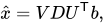
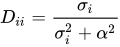
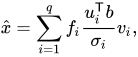
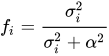
Finally, it is related to the Wiener filter: $${\displaystyle {\hat {x}}=\sum _{i=1}^{q}f_{i}{\frac {u_{i}^{\mathsf {T}}b}{\sigma _{i}}}v_{i},}$$ where the Wiener weights are ${\displaystyle f_{i}={\frac {\sigma _{i}^{2}}{\sigma _{i}^{2}+\alpha ^{2}}}}$ and ${\displaystyle q}$ is the rank of ${\displaystyle A}$.

The optimal regularization parameter ${\displaystyle \alpha }$ is usually unknown and often in practical problems is determined by an ad hoc method. A possible approach relies on the Bayesian interpretation described below. Other approaches include the discrepancy principle, cross-validation, L-curve method,^[26] restricted maximum likelihood and unbiased predictive risk estimator. Grace Wahba proved that the optimal parameter, in the sense of leave-one-out cross-validation minimizes^[27][28] $${\displaystyle G={\frac {\operatorname {RSS} }{\tau ^{2}}}={\frac {\left\|X{\hat {\beta }}-y\right\|^{2}}{\left[\operatorname {Tr} \left(I-X\left(X^{\mathsf {T}}X+\alpha ^{2}I\right)^{-1}X^{\mathsf {T}}\right)\right]^{2}}},}$$ where ${\displaystyle \operatorname {RSS} }$ is the residual sum of squares, and ${\displaystyle \tau }$ is the effective number of degrees of freedom.

Using the previous SVD decomposition, we can simplify the above expression: $${\displaystyle \operatorname {RSS} =\left\|y-\sum _{i=1}^{q}(u_{i}'b)u_{i}\right\|^{2}+\left\|\sum _{i=1}^{q}{\frac {\alpha ^{2}}{\sigma _{i}^{2}+\alpha ^{2}}}(u_{i}'b)u_{i}\right\|^{2},}$$ $${\displaystyle \operatorname {RSS} =\operatorname {RSS} _{0}+\left\|\sum _{i=1}^{q}{\frac {\alpha ^{2}}{\sigma _{i}^{2}+\alpha ^{2}}}(u_{i}'b)u_{i}\right\|^{2},}$$ and $${\displaystyle \tau =m-\sum _{i=1}^{q}{\frac {\sigma _{i}^{2}}{\sigma _{i}^{2}+\alpha ^{2}}}=m-q+\sum _{i=1}^{q}{\frac {\alpha ^{2}}{\sigma _{i}^{2}+\alpha ^{2}}}.}$$

The probabilistic formulation of an inverse problem introduces (when all uncertainties are Gaussian) a covariance matrix ${\displaystyle C_{M}}$ representing the a priori uncertainties on the model parameters, and a covariance matrix ${\displaystyle C_{D}}$ representing the uncertainties on the observed parameters.^[29] In the special case when these two matrices are diagonal and isotropic, ${\displaystyle C_{M}=\sigma _{M}^{2}I}$ and ${\displaystyle C_{D}=\sigma _{D}^{2}I}$, and, in this case, the equations of inverse theory reduce to the equations above, with ${\displaystyle \alpha ={\sigma _{D}}/{\sigma _{M}}}$.^[30][31]

Although at first the choice of the solution to this regularized problem may look artificial, and indeed the matrix ${\displaystyle \Gamma }$ seems rather arbitrary, the process can be justified from a Bayesian point of view.^[32] Note that for an ill-posed problem one must necessarily introduce some additional assumptions in order to get a unique solution. Statistically, the prior probability distribution of ${\displaystyle x}$ is sometimes taken to be a multivariate normal distribution.^[33] For simplicity here, the following assumptions are made: the means are zero; their components are independent; the components have the same standard deviation ${\displaystyle \sigma _{x}}$. The data are also subject to errors, and the errors in ${\displaystyle b}$ are also assumed to be independent with zero mean and standard deviation ${\displaystyle \sigma _{b}}$. Under these assumptions the Tikhonov-regularized solution is the most probable solution given the data and the a priori distribution of ${\displaystyle x}$, according to Bayes' theorem.^[34]

If the assumption of normality is replaced by assumptions of homoscedasticity and uncorrelatedness of errors, and if one still assumes zero mean, then the Gauss–Markov theorem entails that the solution is the minimal unbiased linear estimator.^[35]

• LASSO estimator is another regularization method in statistics.
• Elastic net regularization
• Matrix regularization
• L-curve

References

[edit]- ^ a b Hilt, Donald E.; Seegrist, Donald W. (1977). Ridge, a computer program for calculating ridge regression estimates. doi:10.5962/bhl.title.68934.[page needed]
- ^ a b Gruber, Marvin (1998). Improving Efficiency by Shrinkage: The James--Stein and Ridge Regression Estimators. CRC Press. p. 2. ISBN 978-0-8247-0156-7.
- ^ Kennedy, Peter (2003). A Guide to Econometrics (Fifth ed.). Cambridge: The MIT Press. pp. 205–206. ISBN 0-262-61183-X.
- ^ Gruber, Marvin (1998). Improving Efficiency by Shrinkage: The James–Stein and Ridge Regression Estimators. Boca Raton: CRC Press. pp. 7–15. ISBN 0-8247-0156-9.
- ^ Hoerl, Arthur E.; Kennard, Robert W. (1970). "Ridge Regression: Biased Estimation for Nonorthogonal Problems". Technometrics. 12 (1): 55–67. doi:10.2307/1267351. JSTOR 1267351.
- ^ Hoerl, Arthur E.; Kennard, Robert W. (1970). "Ridge Regression: Applications to Nonorthogonal Problems". Technometrics. 12 (1): 69–82. doi:10.2307/1267352. JSTOR 1267352.
- ^ Jolliffe, I. T. (2006). Principal Component Analysis. Springer Science & Business Media. p. 178. ISBN 978-0-387-22440-4.
- ^ For the choice of in practice, see Khalaf, Ghadban; Shukur, Ghazi (2005). "Choosing Ridge Parameter for Regression Problems". Communications in Statistics – Theory and Methods. 34 (5): 1177–1182. doi:10.1081/STA-200056836. S2CID 122983724.
- ^ van Wieringen, Wessel (2021-05-31). "Lecture notes on ridge regression". arXiv:1509.09169 [stat.ME].
- ^ Tikhonov, Andrey Nikolayevich (1943). "Об устойчивости обратных задач" [On the stability of inverse problems]. Doklady Akademii Nauk SSSR. 39 (5): 195–198. Archived from the original on 2005-02-27.
- ^ Tikhonov, A. N. (1963). "О решении некорректно поставленных задач и методе регуляризации". Doklady Akademii Nauk SSSR. 151: 501–504.. Translated in "Solution of incorrectly formulated problems and the regularization method". Soviet Mathematics. 4: 1035–1038.
- ^ Tikhonov, A. N.; V. Y. Arsenin (1977). Solution of Ill-posed Problems. Washington: Winston & Sons. ISBN 0-470-99124-0.
- ^ Tikhonov, Andrey Nikolayevich; Goncharsky, A.; Stepanov, V. V.; Yagola, Anatolij Grigorevic (30 June 1995). Numerical Methods for the Solution of Ill-Posed Problems. Netherlands: Springer Netherlands. ISBN 0-7923-3583-X. Retrieved 9 August 2018.
- ^ Tikhonov, Andrey Nikolaevich; Leonov, Aleksandr S.; Yagola, Anatolij Grigorevic (1998). Nonlinear ill-posed problems. London: Chapman & Hall. ISBN 0-412-78660-5. Retrieved 9 August 2018.
- ^ Phillips, D. L. (1962). "A Technique for the Numerical Solution of Certain Integral Equations of the First Kind". Journal of the ACM. 9: 84–97. doi:10.1145/321105.321114. S2CID 35368397.
- ^ Hoerl, Arthur E. (1962). "Application of Ridge Analysis to Regression Problems". Chemical Engineering Progress. 58 (3): 54–59.
- ^ Foster, M. (1961). "An Application of the Wiener-Kolmogorov Smoothing Theory to Matrix Inversion". Journal of the Society for Industrial and Applied Mathematics. 9 (3): 387–392. doi:10.1137/0109031.
- ^ Hoerl, A. E.; R. W. Kennard (1970). "Ridge regression: Biased estimation for nonorthogonal problems". Technometrics. 12 (1): 55–67. doi:10.1080/00401706.1970.10488634.
- ^ Hoerl, Roger W. (2020-10-01). "Ridge Regression: A Historical Context". Technometrics. 62 (4): 420–425. doi:10.1080/00401706.2020.1742207. ISSN 0040-1706.
- ^ Ng, Andrew Y. (2004). Feature selection, L1 vs. L2 regularization, and rotational invariance (PDF). Proc. ICML.
- ^ R.-E. Fan; K.-W. Chang; C.-J. Hsieh; X.-R. Wang; C.-J. Lin (2008). "LIBLINEAR: A library for large linear classification". Journal of Machine Learning Research. 9: 1871–1874.
- ^ Guan, Naiyang; Tao, Dacheng; Luo, Zhigang; Yuan, Bo (2012). "Online nonnegative matrix factorization with robust stochastic approximation". IEEE Transactions on Neural Networks and Learning Systems. 23 (7): 1087–1099. Bibcode:2012ITNNL..23.1087G. doi:10.1109/TNNLS.2012.2197827. PMID 24807135. S2CID 8755408.
- ^ Koch, Lukas (2022). "Post-hoc regularisation of unfolded cross-section measurements". Journal of Instrumentation. 17 (10) 10021. arXiv:2207.02125. Bibcode:2022JInst..17P0021K. doi:10.1088/1748-0221/17/10/P10021.
- ^ Lavrentiev, M. M. (1967). Some Improperly Posed Problems of Mathematical Physics. New York: Springer.
- ^ Hansen, Per Christian (Jan 1, 1998). Rank-Deficient and Discrete Ill-Posed Problems: Numerical Aspects of Linear Inversion (1st ed.). Philadelphia, USA: SIAM. ISBN 978-0-89871-403-6.
- ^ P. C. Hansen, "The L-curve and its use in the numerical treatment of inverse problems", [1]
- ^ Wahba, G. (1990). "Spline Models for Observational Data". CBMS-NSF Regional Conference Series in Applied Mathematics. Society for Industrial and Applied Mathematics. Bibcode:1990smod.conf.....W.
- ^ Golub, G.; Heath, M.; Wahba, G. (1979). "Generalized cross-validation as a method for choosing a good ridge parameter" (PDF). Technometrics. 21 (2): 215–223. doi:10.1080/00401706.1979.10489751.
- ^ Tarantola, Albert (2005). Inverse Problem Theory and Methods for Model Parameter Estimation (1st ed.). Philadelphia: Society for Industrial and Applied Mathematics (SIAM). ISBN 0-89871-792-2. Retrieved 9 August 2018.
- ^ Huang, Yunfei.; et al. (2019). "Traction force microscopy with optimized regularization and automated Bayesian parameter selection for comparing cells". Scientific Reports. 9 (1) 539: 537. arXiv:1810.05848. Bibcode:2019NatSR...9..539H. doi:10.1038/s41598-018-36896-x. PMC 6345967. PMID 30679578.
- ^ Huang, Yunfei; Gompper, Gerhard; Sabass, Benedikt (2020). "A Bayesian traction force microscopy method with automated denoising in a user-friendly software package". Computer Physics Communications. 256 107313. arXiv:2005.01377. Bibcode:2020CoPhC.25607313H. doi:10.1016/j.cpc.2020.107313.
- ^ Greenberg, Edward; Webster, Charles E. Jr. (1983). Advanced Econometrics: A Bridge to the Literature. New York: John Wiley & Sons. pp. 207–213. ISBN 0-471-09077-8.
- ^ Vogel, Curtis R. (2002). Computational methods for inverse problems. Philadelphia: Society for Industrial and Applied Mathematics. ISBN 0-89871-550-4.
- ^ Amemiya, Takeshi (1985). Advanced Econometrics. Harvard University Press. pp. 60–61. ISBN 0-674-00560-0.
Further reading
[edit]- Gruber, Marvin (1998). Improving Efficiency by Shrinkage: The James–Stein and Ridge Regression Estimators. Boca Raton: CRC Press. ISBN 0-8247-0156-9.
- Kress, Rainer (1998). "Tikhonov Regularization". Numerical Analysis. New York: Springer. pp. 86–90. ISBN 0-387-98408-9.
- Press, W. H.; Teukolsky, S. A.; Vetterling, W. T.; Flannery, B. P. (2007). "Section 19.5. Linear Regularization Methods". Numerical Recipes: The Art of Scientific Computing (3rd ed.). New York: Cambridge University Press. ISBN 978-0-521-88068-8.
- Saleh, A. K. Md. Ehsanes; Arashi, Mohammad; Kibria, B. M. Golam (2019). Theory of Ridge Regression Estimation with Applications. New York: John Wiley & Sons. ISBN 978-1-118-64461-4.
- Taddy, Matt (2019). "Regularization". Business Data Science: Combining Machine Learning and Economics to Optimize, Automate, and Accelerate Business Decisions. New York: McGraw-Hill. pp. 69–104. ISBN 978-1-260-45277-8.