A linear differential equation or a system of linear equations such that the associated homogeneous equations have constant coefficients may be solved by quadrature, which means that the solutions may be expressed in terms of integrals. This is also true for a linear equation of order one, with non-constant coefficients. An equation of order two or higher with non-constant coefficients cannot, in general, be solved by quadrature. For order two, Kovacic's algorithm allows deciding whether there are solutions in terms of integrals, and computing them if any.

The solutions of homogeneous linear differential equations with polynomial coefficients are called holonomic functions. This class of functions is stable under sums, products, differentiation, integration, and contains many usual functions and special functions such as exponential function, logarithm, sine, cosine, inverse trigonometric functions, error function, Bessel functions and hypergeometric functions. Their representation by the defining differential equation and initial conditions allows making algorithmic (on these functions) most operations of calculus, such as computation of antiderivatives, limits, asymptotic expansion, and numerical evaluation to any precision, with a certified error bound.

The highest order of derivation that appears in a (linear) differential equation is the order of the equation. The term b(x), which does not depend on the unknown function and its derivatives, is sometimes called the constant term of the equation (by analogy with algebraic equations), even when this term is a non-constant function. If the constant term is the zero function, then the differential equation is said to be homogeneous, as it is a homogeneous polynomial in the unknown function and its derivatives. The equation obtained by replacing, in a linear differential equation, the constant term by the zero function is the associated homogeneous equation. A differential equation has constant coefficients if only constant functions appear as coefficients in the associated homogeneous equation.

A solution of a differential equation is a function that satisfies the equation. The solutions of a homogeneous linear differential equation form a vector space. In the ordinary case, this vector space has a finite dimension, equal to the order of the equation. All solutions of a linear differential equation are found by adding to a particular solution any solution of the associated homogeneous equation.

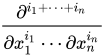
A basic differential operator of order i is a mapping that maps any differentiable function to its ith derivative, or, in the case of several variables, to one of its partial derivatives of order i. It is commonly denoted $${\displaystyle {\frac {d^{i}}{dx^{i}}}}$$ in the case of univariate functions, and $${\displaystyle {\frac {\partial ^{i_{1}+\cdots +i_{n}}}{\partial x_{1}^{i_{1}}\cdots \partial x_{n}^{i_{n}}}}}$$ in the case of functions of n variables. The basic differential operators include the derivative of order 0, which is the identity mapping.

A linear differential operator (abbreviated, in this article, as linear operator or, simply, operator) is a linear combination of basic differential operators, with differentiable functions as coefficients. In the univariate case, a linear operator has thus the form^[1] $${\displaystyle a_{0}(x)+a_{1}(x){\frac {d}{dx}}+\cdots +a_{n}(x){\frac {d^{n}}{dx^{n}}},}$$ where a₀(x), ..., a_n(x) are differentiable functions, and the nonnegative integer n is the order of the operator (if a_n(x) is not the zero function).

Let L be a linear differential operator. The application of L to a function f is usually denoted Lf or Lf(X), if one needs to specify the variable (this must not be confused with a multiplication). A linear differential operator is a linear operator, since it maps sums to sums and the product by a scalar to the product by the same scalar.

As the sum of two linear operators is a linear operator, as well as the product (on the left) of a linear operator by a differentiable function, the linear differential operators form a vector space over the real numbers or the complex numbers (depending on the nature of the functions that are considered). They form also a free module over the ring of differentiable functions.

The language of operators allows a compact writing for differentiable equations: if $${\displaystyle L=a_{0}(x)+a_{1}(x){\frac {d}{dx}}+\cdots +a_{n}(x){\frac {d^{n}}{dx^{n}}},}$$ is a linear differential operator, then the equation $${\displaystyle a_{0}(x)y+a_{1}(x)y'+a_{2}(x)y''+\cdots +a_{n}(x)y^{(n)}=b(x)}$$ may be rewritten $${\displaystyle Ly=b(x).}$$

There may be several variants to this notation; in particular the variable of differentiation may appear explicitly or not in y and the right-hand and of the equation, such as Ly(x) = b(x) or Ly = b.

The kernel of a linear differential operator is its kernel as a linear mapping, that is the vector space of the solutions of the (homogeneous) differential equation Ly = 0.

In the case of an ordinary differential operator of order n, Carathéodory's existence theorem implies that, under very mild conditions, the kernel of L is a vector space of dimension n, and that the solutions of the equation Ly(x) = b(x) have the form $${\displaystyle S_{0}(x)+c_{1}S_{1}(x)+\cdots +c_{n}S_{n}(x),}$$ where c₁, ..., c_n are arbitrary numbers. Typically, the hypotheses of Carathéodory's theorem are satisfied in an interval I, if the functions b, a₀, ..., a_n are continuous in I, and there is a positive real number k such that |a_n(x)| > k for every x in I.

A homogeneous linear differential equation has constant coefficients if it has the form $${\displaystyle a_{0}y+a_{1}y'+a_{2}y''+\cdots +a_{n}y^{(n)}=0}$$ where a₁, ..., a_n are (real or complex) numbers. In other words, it has constant coefficients if it is defined by a linear operator with constant coefficients.

The study of these differential equations with constant coefficients dates back to Leonhard Euler, who introduced the exponential function ${\displaystyle e^{x}}$, which is the unique solution of the equation ${\displaystyle f'=f}$, such that ${\displaystyle f(0)=1}$. It follows that the nth derivative of ${\displaystyle e^{cx}}$ is ${\displaystyle c^{n}e^{cx}}$, and this allows solving homogeneous linear differential equations rather easily.

Let $${\displaystyle a_{0}y+a_{1}y'+a_{2}y''+\cdots +a_{n}y^{(n)}=0}$$ be a homogeneous linear differential equation with constant coefficients (that is a₀, ..., a_n are real or complex numbers).

Searching solutions of this equation that have the form e^αx is equivalent to searching the constants α such that $${\displaystyle a_{0}e^{\alpha x}+a_{1}\alpha e^{\alpha x}+a_{2}\alpha ^{2}e^{\alpha x}+\cdots +a_{n}\alpha ^{n}e^{\alpha x}=0.}$$ Factoring out e^αx (which is never zero), shows that α must be a root of the characteristic polynomial $${\displaystyle a_{0}+a_{1}t+a_{2}t^{2}+\cdots +a_{n}t^{n}}$$ of the differential equation, which is the left-hand side of the characteristic equation $${\displaystyle a_{0}+a_{1}t+a_{2}t^{2}+\cdots +a_{n}t^{n}=0.}$$

When these roots are all distinct, one has n distinct solutions that are not necessarily real, even if the coefficients of the equation are real. These solutions can be shown to be linearly independent, by considering the Vandermonde determinant of the values of these solutions at x = 0, ..., n – 1. Together they form a basis of the vector space of solutions of the differential equation (that is, the kernel of the differential operator).

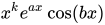
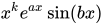
In the case where the characteristic polynomial has only simple roots, the preceding provides a complete basis of the solutions vector space. In the case of multiple roots, more linearly independent solutions are needed for having a basis. These have the form $${\displaystyle x^{k}e^{\alpha x},}$$ where k is a nonnegative integer, α is a root of the characteristic polynomial of multiplicity m, and k < m. For proving that these functions are solutions, one may remark that if α is a root of the characteristic polynomial of multiplicity m, the characteristic polynomial may be factored as P(t)(t − α)^m. Thus, applying the differential operator of the equation is equivalent with applying first m times the operator ${\textstyle {\frac {d}{dx}}-\alpha }$, and then the operator that has P as characteristic polynomial. By the exponential shift theorem, $${\displaystyle \left({\frac {d}{dx}}-\alpha \right)\left(x^{k}e^{\alpha x}\right)=kx^{k-1}e^{\alpha x},}$$

and thus one gets zero after k + 1 application of ${\textstyle {\frac {d}{dx}}-\alpha }$.

As, by the fundamental theorem of algebra, the sum of the multiplicities of the roots of a polynomial equals the degree of the polynomial, the number of above solutions equals the order of the differential equation, and these solutions form a basis of the vector space of the solutions.

In the common case where the coefficients of the equation are real, it is generally more convenient to have a basis of the solutions consisting of real-valued functions. Such a basis may be obtained from the preceding basis by remarking that, if a + ib is a root of the characteristic polynomial, then a – ib is also a root, of the same multiplicity. Thus a real basis is obtained by using Euler's formula, and replacing ${\displaystyle x^{k}e^{(a+ib)x}}$ and ${\displaystyle x^{k}e^{(a-ib)x}}$ by ${\displaystyle x^{k}e^{ax}\cos(bx)}$ and ${\displaystyle x^{k}e^{ax}\sin(bx)}$.

A homogeneous linear differential equation of the second order may be written $${\displaystyle y''+ay'+by=0,}$$ and its characteristic polynomial is $${\displaystyle r^{2}+ar+b.}$$

If a and b are real, there are three cases for the solutions, depending on the discriminant D = a² − 4b. In all three cases, the general solution depends on two arbitrary constants c₁ and c₂.

• If D > 0, the characteristic polynomial has two distinct real roots α, and β. In this case, the general solution is $${\displaystyle c_{1}e^{\alpha x}+c_{2}e^{\beta x}.}$$
• If D = 0, the characteristic polynomial has a double root −a/2, and the general solution is $${\displaystyle (c_{1}+c_{2}x)e^{-ax/2}.}$$
• If D < 0, the characteristic polynomial has two complex conjugate roots α ± βi, and the general solution is $${\displaystyle c_{1}e^{(\alpha +\beta i)x}+c_{2}e^{(\alpha -\beta i)x},}$$ which may be rewritten in real terms, using Euler's formula as $${\displaystyle e^{\alpha x}(c_{1}\cos(\beta x)+c_{2}\sin(\beta x)).}$$

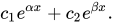
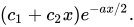
Finding the solution y(x) satisfying y(0) = d₁ and y′(0) = d₂, one equates the values of the above general solution at 0 and its derivative there to d₁ and d₂, respectively. This results in a linear system of two linear equations in the two unknowns c₁ and c₂. Solving this system gives the solution for a so-called Cauchy problem, in which the values at 0 for the solution of the DEQ and its derivative are specified.

A non-homogeneous equation of order n with constant coefficients may be written $${\displaystyle y^{(n)}(x)+a_{1}y^{(n-1)}(x)+\cdots +a_{n-1}y'(x)+a_{n}y(x)=f(x),}$$ where a₁, ..., a_n are real or complex numbers, f is a given function of x, and y is the unknown function (for sake of simplicity, "(x)" will be omitted in the following).

There are several methods for solving such an equation. The best method depends on the nature of the function f that makes the equation non-homogeneous. If f is a linear combination of exponential and sinusoidal functions, then the exponential response formula may be used. If, more generally, f is a linear combination of functions of the form xⁿe^ax, xⁿ cos(ax), and xⁿ sin(ax), where n is a nonnegative integer, and a a constant (which need not be the same in each term), then the method of undetermined coefficients may be used. Still more general, the annihilator method applies when f satisfies a homogeneous linear differential equation, typically, a holonomic function.

The most general method is the variation of constants, which is presented here.

The general solution of the associated homogeneous equation $${\displaystyle y^{(n)}+a_{1}y^{(n-1)}+\cdots +a_{n-1}y'+a_{n}y=0}$$ is $${\displaystyle y=u_{1}y_{1}+\cdots +u_{n}y_{n},}$$ where (y₁, ..., y_n) is a basis of the vector space of the solutions and u₁, ..., u_n are arbitrary constants. The method of variation of constants takes its name from the following idea. Instead of considering u₁, ..., u_n as constants, they can be considered as unknown functions that have to be determined for making y a solution of the non-homogeneous equation. For this purpose, one adds the constraints $${\displaystyle {\begin{aligned}0&=u'_{1}y_{1}+u'_{2}y_{2}+\cdots +u'_{n}y_{n}\\0&=u'_{1}y'_{1}+u'_{2}y'_{2}+\cdots +u'_{n}y'_{n}\\&\;\;\vdots \\0&=u'_{1}y_{1}^{(n-2)}+u'_{2}y_{2}^{(n-2)}+\cdots +u'_{n}y_{n}^{(n-2)},\end{aligned}}}$$ which imply (by product rule and induction) $${\displaystyle y^{(i)}=u_{1}y_{1}^{(i)}+\cdots +u_{n}y_{n}^{(i)}}$$ for i = 1, ..., n – 1, and $${\displaystyle y^{(n)}=u_{1}y_{1}^{(n)}+\cdots +u_{n}y_{n}^{(n)}+u'_{1}y_{1}^{(n-1)}+u'_{2}y_{2}^{(n-1)}+\cdots +u'_{n}y_{n}^{(n-1)}.}$$

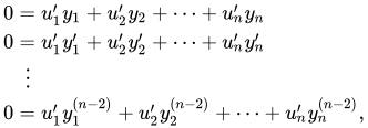
Replacing in the original equation y and its derivatives by these expressions, and using the fact that y₁, ..., y_n are solutions of the original homogeneous equation, one gets $${\displaystyle f=u'_{1}y_{1}^{(n-1)}+\cdots +u'_{n}y_{n}^{(n-1)}.}$$

This equation and the above ones with 0 as left-hand side form a system of n linear equations in u′₁, ..., u′_n whose coefficients are known functions (f, the y_i, and their derivatives). This system can be solved by any method of linear algebra. The computation of antiderivatives gives u₁, ..., u_n, and then y = u₁y₁ + ⋯ + u_ny_n.

As antiderivatives are defined up to the addition of a constant, one finds again that the general solution of the non-homogeneous equation is the sum of an arbitrary solution and the general solution of the associated homogeneous equation.

The general form of a linear ordinary differential equation of order 1, after dividing out the coefficient of y′(x), is: $${\displaystyle y'(x)=f(x)y(x)+g(x).}$$

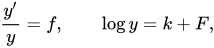
If the equation is homogeneous, i.e. g(x) = 0, one may rewrite and integrate: $${\displaystyle {\frac {y'}{y}}=f,\qquad \log y=k+F,}$$ where k is an arbitrary constant of integration and ${\displaystyle F=\textstyle \int f\,dx}$ is any antiderivative of f. Thus, the general solution of the homogeneous equation is $${\displaystyle y=ce^{F},}$$ where c = e^k is an arbitrary constant.

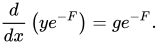
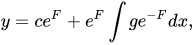
For the general non-homogeneous equation, it is useful to multiply both sides of the equation by the reciprocal e^−F of a solution of the homogeneous equation.^[2] This gives $${\displaystyle y'e^{-F}-yfe^{-F}=ge^{-F}.}$$ As ⁠${\displaystyle -fe^{-F}={\tfrac {d}{dx}}\left(e^{-F}\right),}$⁠ the product rule allows rewriting the equation as $${\displaystyle {\frac {d}{dx}}\left(ye^{-F}\right)=ge^{-F}.}$$ Thus, the general solution is $${\displaystyle y=ce^{F}+e^{F}\int ge^{-F}dx,}$$ where c is a constant of integration, and F is any antiderivative of f (changing of antiderivative amounts to change the constant of integration).

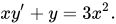
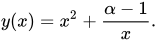
Solving the equation $${\displaystyle y'(x)+{\frac {y(x)}{x}}=3x.}$$ The associated homogeneous equation ${\displaystyle y'(x)+{\frac {y(x)}{x}}=0}$ gives $${\displaystyle {\frac {y'}{y}}=-{\frac {1}{x}},}$$ that is $${\displaystyle y={\frac {c}{x}}.}$$

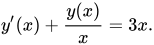
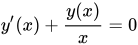
Dividing the original equation by one of these solutions gives $${\displaystyle xy'+y=3x^{2}.}$$ That is $${\displaystyle (xy)'=3x^{2},}$$ $${\displaystyle xy=x^{3}+c,}$$ and $${\displaystyle y(x)=x^{2}+c/x.}$$ For the initial condition $${\displaystyle y(1)=\alpha ,}$$ one gets the particular solution $${\displaystyle y(x)=x^{2}+{\frac {\alpha -1}{x}}.}$$

A system of linear differential equations consists of several linear differential equations that involve several unknown functions. In general one restricts the study to systems such that the number of unknown functions equals the number of equations.

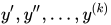
An arbitrary linear ordinary differential equation and a system of such equations can be converted into a first order system of linear differential equations by adding variables for all but the highest order derivatives. That is, if ⁠${\displaystyle y',y'',\ldots ,y^{(k)}}$⁠ appear in an equation, one may replace them by new unknown functions ⁠${\displaystyle y_{1},\ldots ,y_{k}}$⁠ that must satisfy the equations ⁠${\displaystyle y'=y_{1}}$⁠ and ⁠${\displaystyle y_{i}'=y_{i+1},}$⁠ for i = 1, ..., k – 1.

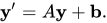
A linear system of the first order, which has n unknown functions and n differential equations may normally be solved for the derivatives of the unknown functions. If it is not the case this is a differential-algebraic system, and this is a different theory. Therefore, the systems that are considered here have the form $${\displaystyle {\begin{aligned}y_{1}'(x)&=b_{1}(x)+a_{1,1}(x)y_{1}+\cdots +a_{1,n}(x)y_{n}\\[1ex]&\;\;\vdots \\[1ex]y_{n}'(x)&=b_{n}(x)+a_{n,1}(x)y_{1}+\cdots +a_{n,n}(x)y_{n},\end{aligned}}}$$ where ⁠${\displaystyle b_{n}}$⁠ and the ⁠${\displaystyle a_{i,j}}$⁠ are functions of x. In matrix notation, this system may be written (omitting "(x)") $${\displaystyle \mathbf {y} '=A\mathbf {y} +\mathbf {b} .}$$

The solving method is similar to that of a single first order linear differential equations, but with complications stemming from noncommutativity of matrix multiplication.

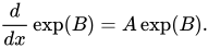
Let $${\displaystyle \mathbf {u} '=A\mathbf {u} .}$$ be the homogeneous equation associated to the above matrix equation. Its solutions form a vector space of dimension n, and are therefore the columns of a square matrix of functions ⁠${\displaystyle U(x)}$⁠, whose determinant is not the zero function. If n = 1, or A is a matrix of constants, or, more generally, if A commutes with its antiderivative ⁠${\displaystyle \textstyle B=\int Adx}$⁠, then one may choose U equal the exponential of B. In fact, in these cases, one has $${\displaystyle {\frac {d}{dx}}\exp(B)=A\exp(B).}$$ In the general case there is no closed-form solution for the homogeneous equation, and one has to use either a numerical method, or an approximation method such as Magnus expansion.

Knowing the matrix U, the general solution of the non-homogeneous equation is $${\displaystyle \mathbf {y} (x)=U(x)\mathbf {y_{0}} +U(x)\int U^{-1}(x)\mathbf {b} (x)\,dx,}$$ where the column matrix ${\displaystyle \mathbf {y_{0}} }$ is an arbitrary constant of integration.

If initial conditions are given as $${\displaystyle \mathbf {y} (x_{0})=\mathbf {y} _{0},}$$ the solution that satisfies these initial conditions is $${\displaystyle \mathbf {y} (x)=U(x)U^{-1}(x_{0})\mathbf {y_{0}} +U(x)\int _{x_{0}}^{x}U^{-1}(t)\mathbf {b} (t)\,dt.}$$

A linear ordinary equation of order one with variable coefficients may be solved by quadrature, which means that the solutions may be expressed in terms of integrals. This is not the case for order at least two. This is the main result of Picard–Vessiot theory which was initiated by Émile Picard and Ernest Vessiot, and whose recent developments are called differential Galois theory.

The impossibility of solving by quadrature can be compared with the Abel–Ruffini theorem, which states that an algebraic equation of degree at least five cannot, in general, be solved by radicals. This analogy extends to the proof methods and motivates the denomination of differential Galois theory.

Similarly to the algebraic case, the theory allows deciding which equations may be solved by quadrature, and if possible solving them. However, for both theories, the necessary computations are extremely difficult, even with the most powerful computers.

Nevertheless, the case of order two with rational coefficients has been completely solved by Kovacic's algorithm.

Cauchy–Euler equations are examples of equations of any order, with variable coefficients, that can be solved explicitly. These are the equations of the form $${\displaystyle x^{n}y^{(n)}(x)+a_{n-1}x^{n-1}y^{(n-1)}(x)+\cdots +a_{0}y(x)=0,}$$ where ⁠${\displaystyle a_{0},\ldots ,a_{n-1}}$⁠ are constant coefficients.

A holonomic function, also called a D-finite function, is a function that is a solution of a homogeneous linear differential equation with polynomial coefficients.

Most functions that are commonly considered in mathematics are holonomic or quotients of holonomic functions. In fact, holonomic functions include polynomials, algebraic functions, logarithm, exponential function, sine, cosine, hyperbolic sine, hyperbolic cosine, inverse trigonometric and inverse hyperbolic functions, and many special functions such as Bessel functions and hypergeometric functions.

Holonomic functions have several closure properties; in particular, sums, products, derivative and integrals of holonomic functions are holonomic. Moreover, these closure properties are effective, in the sense that there are algorithms for computing the differential equation of the result of any of these operations, knowing the differential equations of the input.^[3]

Usefulness of the concept of holonomic functions results of Zeilberger's theorem, which follows.^[3]

A holonomic sequence is a sequence of numbers that may be generated by a recurrence relation with polynomial coefficients. The coefficients of the Taylor series at a point of a holonomic function form a holonomic sequence. Conversely, if the sequence of the coefficients of a power series is holonomic, then the series defines a holonomic function (even if the radius of convergence is zero). There are efficient algorithms for both conversions, that is for computing the recurrence relation from the differential equation, and vice versa. ^[3]

It follows that, if one represents (in a computer) holonomic functions by their defining differential equations and initial conditions, most calculus operations can be done automatically on these functions, such as derivative, indefinite and definite integral, fast computation of Taylor series (thanks of the recurrence relation on its coefficients), evaluation to a high precision with certified bound of the approximation error, limits, localization of singularities, asymptotic behavior at infinity and near singularities, proof of identities, etc.^[4]

• Continuous-repayment mortgage
• Fourier transform
• Laplace transform
• Linear difference equation
• Variation of parameters