System of linear equations

The system of one equation in one unknown

${\displaystyle 2x=4}$

has the solution

${\displaystyle x=2.}$

However, most interesting linear systems have at least two equations.

The simplest kind of nontrivial linear system involves two equations and two variables:

${\displaystyle {\begin{alignedat}{5}2x&&\;+\;&&3y&&\;=\;&&6&\\4x&&\;+\;&&9y&&\;=\;&&15&.\end{alignedat}}}$

One method for solving such a system is as follows. First, solve the top equation for ${\displaystyle x}$ in terms of ${\displaystyle y}$:

${\displaystyle x=3-{\frac {3}{2}}y.}$

Now substitute this expression for x into the bottom equation:

${\displaystyle 4\left(3-{\frac {3}{2}}y\right)+9y=15.}$

This results in a single equation involving only the variable ${\displaystyle y}$. Solving gives ${\displaystyle y=1}$, and substituting this back into the equation for ${\displaystyle x}$ yields ${\displaystyle x={\frac {3}{2}}}$. This method generalizes to systems with additional variables (see "elimination of variables" below, or the article on elementary algebra.)

A general system of m linear equations with n unknowns and coefficients can be written as

${\displaystyle {\begin{cases}a_{11}x_{1}+a_{12}x_{2}+\dots +a_{1n}x_{n}=b_{1}\\a_{21}x_{1}+a_{22}x_{2}+\dots +a_{2n}x_{n}=b_{2}\\\vdots \\a_{m1}x_{1}+a_{m2}x_{2}+\dots +a_{mn}x_{n}=b_{m},\end{cases}}}$

where ${\displaystyle x_{1},x_{2},\dots ,x_{n}}$ are the unknowns, ${\displaystyle a_{11},a_{12},\dots ,a_{mn}}$ are the coefficients of the system, and ${\displaystyle b_{1},b_{2},\dots ,b_{m}}$ are the constant terms.^[3]

Often the coefficients and unknowns are real or complex numbers, but integers and rational numbers are also seen, as are polynomials and elements of an abstract algebraic structure.

One extremely helpful view is that each unknown is a weight for a column vector in a linear combination.

${\displaystyle x_{1}{\begin{bmatrix}a_{11}\\a_{21}\\\vdots \\a_{m1}\end{bmatrix}}+x_{2}{\begin{bmatrix}a_{12}\\a_{22}\\\vdots \\a_{m2}\end{bmatrix}}+\dots +x_{n}{\begin{bmatrix}a_{1n}\\a_{2n}\\\vdots \\a_{mn}\end{bmatrix}}={\begin{bmatrix}b_{1}\\b_{2}\\\vdots \\b_{m}\end{bmatrix}}}$

This allows all the language and theory of vector spaces (or more generally, modules) to be brought to bear. For example, the collection of all possible linear combinations of the vectors on the left-hand side (LHS) is called their span, and the equations have a solution just when the right-hand vector is within that span. If every vector within that span has exactly one expression as a linear combination of the given left-hand vectors, then any solution is unique. In any event, the span has a basis of linearly independent vectors that do guarantee exactly one expression; and the number of vectors in that basis (its dimension) cannot be larger than m or n, but it can be smaller. This is important because if we have m independent vectors a solution is guaranteed regardless of the right-hand side (RHS), and otherwise not guaranteed.

The vector equation is equivalent to a matrix equation of the form $${\displaystyle A\mathbf {x} =\mathbf {b} }$$ where A is an m×n matrix, x is a column vector with n entries, and b is a column vector with m entries.^[4]

$${\displaystyle A={\begin{bmatrix}a_{11}&a_{12}&\cdots &a_{1n}\\a_{21}&a_{22}&\cdots &a_{2n}\\\vdots &\vdots &\ddots &\vdots \\a_{m1}&a_{m2}&\cdots &a_{mn}\end{bmatrix}},\quad \mathbf {x} ={\begin{bmatrix}x_{1}\\x_{2}\\\vdots \\x_{n}\end{bmatrix}},\quad \mathbf {b} ={\begin{bmatrix}b_{1}\\b_{2}\\\vdots \\b_{m}\end{bmatrix}}.}$$ The number of vectors in a basis for the span of the columns vectors in A is now expressed as the rank of the matrix.

A solution of a linear system is an assignment of values to the variables ${\displaystyle x_{1},x_{2},\dots ,x_{n}}$ such that each of the equations is satisfied. The set of all possible solutions is called the solution set.^[5]

A linear system may behave in any one of three possible ways:

1. The system has infinitely many solutions.
2. The system has a unique solution.
3. The system has no solution.

For a system involving two variables (x and y), each linear equation determines a line on the xy-plane. Because a solution to a linear system must satisfy all of the equations, the solution set is the intersection of these lines, and is hence either a line, a single point, or the empty set.

For three variables, each linear equation determines a plane in three-dimensional space, and the solution set is the intersection of these planes. Thus the solution set may be a plane, a line, a single point, or the empty set. For example, as three parallel planes do not have a common point, the solution set of their equations is empty; the solution set of the equations of three planes intersecting at a point is single point; if three planes pass through two points, their equations have at least two common solutions; in fact the solution set is infinite and consists in all the line passing through these points.^[6]

For n variables, each linear equation determines a hyperplane in n-dimensional space. The solution set is the intersection of these hyperplanes, and is a flat, which may have any dimension lower than n.

In general, the behavior of a linear system is determined by the relationship between the number of equations and the number of unknowns. Here, "in general" means that a different behavior may occur for specific values of the coefficients of the equations.

• In general, a system with fewer equations than unknowns has infinitely many solutions, but it may have no solution. Such a system is known as an underdetermined system.
• In general, a system with the same number of equations and unknowns has a single unique solution.
• In general, a system with more equations than unknowns has no solution. Such a system is also known as an overdetermined system.

In the first case, the dimension of the solution set is, in general, equal to n − m, where n is the number of variables and m is the number of equations.

The following pictures illustrate this trichotomy in the case of two variables:

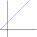
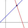
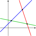
One equation	Two equations	Three equations

The first system has infinitely many solutions, namely all of the points on the blue line. The second system has a single unique solution, namely the intersection of the two lines. The third system has no solutions, since the three lines share no common point.

It must be kept in mind that the pictures above show only the most common case (the general case). It is possible for a system of two equations and two unknowns to have no solution (if the two lines are parallel), or for a system of three equations and two unknowns to be solvable (if the three lines intersect at a single point).

A system of linear equations behave differently from the general case if the equations are linearly dependent, or if it is inconsistent and has no more equations than unknowns.

The equations of a linear system are independent if none of the equations can be derived algebraically from the others. When the equations are independent, each equation contains new information about the variables, and removing any of the equations increases the size of the solution set. For linear equations, logical independence is the same as linear independence.

For example, the equations

${\displaystyle 3x+2y=6\;\;\;\;{\text{and}}\;\;\;\;6x+4y=12}$

are not independent — they are the same equation when scaled by a factor of two, and they would produce identical graphs. This is an example of equivalence in a system of linear equations.

For a more complicated example, the equations

${\displaystyle {\begin{alignedat}{5}x&&\;-\;&&2y&&\;=\;&&-1&\\3x&&\;+\;&&5y&&\;=\;&&8&\\4x&&\;+\;&&3y&&\;=\;&&7&\end{alignedat}}}$

are not independent, because the third equation is the sum of the other two. Indeed, any one of these equations can be derived from the other two, and any one of the equations can be removed without affecting the solution set. The graphs of these equations are three lines that intersect at a single point.

A linear system is inconsistent if it has no solution, and otherwise, it is said to be consistent.^[7] When the system is inconsistent, it is possible to derive a contradiction from the equations, that may always be rewritten as the statement 0 = 1.

For example, the equations

${\displaystyle 3x+2y=6\;\;\;\;{\text{and}}\;\;\;\;3x+2y=12}$

are inconsistent. In fact, by subtracting the first equation from the second one and multiplying both sides of the result by 1/6, we get 0 = 1. The graphs of these equations on the xy-plane are a pair of parallel lines.

It is possible for three linear equations to be inconsistent, even though any two of them are consistent together. For example, the equations

${\displaystyle {\begin{alignedat}{7}x&&\;+\;&&y&&\;=\;&&1&\\2x&&\;+\;&&y&&\;=\;&&1&\\3x&&\;+\;&&2y&&\;=\;&&3&\end{alignedat}}}$

are inconsistent. Adding the first two equations together gives 3x + 2y = 2, which can be subtracted from the third equation to yield 0 = 1. Any two of these equations have a common solution. The same phenomenon can occur for any number of equations.

In general, inconsistencies occur if the left-hand sides of the equations in a system are linearly dependent, and the constant terms do not satisfy the dependence relation. A system of equations whose left-hand sides are linearly independent is always consistent.

Putting it another way, according to the Rouché–Capelli theorem, any system of equations (overdetermined or otherwise) is inconsistent if the rank of the augmented matrix is greater than the rank of the coefficient matrix. If, on the other hand, the ranks of these two matrices are equal, the system must have at least one solution. The solution is unique if and only if the rank equals the number of variables. Otherwise the general solution has k free parameters where k is the difference between the number of variables and the rank; hence in such a case there is an infinitude of solutions. The rank of a system of equations (that is, the rank of the augmented matrix) can never be higher than [the number of variables] + 1, which means that a system with any number of equations can always be reduced to a system that has a number of independent equations that is at most equal to [the number of variables] + 1.

Two linear systems using the same set of variables are equivalent if each of the equations in the second system can be derived algebraically from the equations in the first system, and vice versa. Two systems are equivalent if either both are inconsistent or each equation of each of them is a linear combination of the equations of the other one. It follows that two linear systems are equivalent if and only if they have the same solution set.

There are several algorithms for solving a system of linear equations.

When the solution set is finite, it is reduced to a single element. In this case, the unique solution is described by a sequence of equations whose left-hand sides are the names of the unknowns and right-hand sides are the corresponding values, for example ${\displaystyle (x=3,\;y=-2,\;z=6)}$. When an order on the unknowns has been fixed, for example the alphabetical order the solution may be described as a vector of values, like ${\displaystyle (3,\,-2,\,6)}$ for the previous example.

To describe a set with an infinite number of solutions, typically some of the variables are designated as free (or independent, or as parameters), meaning that they are allowed to take any value, while the remaining variables are dependent on the values of the free variables.

For example, consider the following system:

${\displaystyle {\begin{alignedat}{7}x&&\;+\;&&3y&&\;-\;&&2z&&\;=\;&&5&\\3x&&\;+\;&&5y&&\;+\;&&6z&&\;=\;&&7&\end{alignedat}}}$

The solution set to this system can be described by the following equations:

${\displaystyle x=-7z-1\;\;\;\;{\text{and}}\;\;\;\;y=3z+2{\text{.}}}$

Here z is the free variable, while x and y are dependent on z. Any point in the solution set can be obtained by first choosing a value for z, and then computing the corresponding values for x and y.

Each free variable gives the solution space one degree of freedom, the number of which is equal to the dimension of the solution set. For example, the solution set for the above equation is a line, since a point in the solution set can be chosen by specifying the value of the parameter z. An infinite solution of higher order may describe a plane, or higher-dimensional set.

Different choices for the free variables may lead to different descriptions of the same solution set. For example, the solution to the above equations can alternatively be described as follows:

${\displaystyle y=-{\frac {3}{7}}x+{\frac {11}{7}}\;\;\;\;{\text{and}}\;\;\;\;z=-{\frac {1}{7}}x-{\frac {1}{7}}{\text{.}}}$

Here x is the free variable, and y and z are dependent.

The simplest method for solving a system of linear equations is to repeatedly eliminate variables. This method can be described as follows:

1. In the first equation, solve for one of the variables in terms of the others.
2. Substitute this expression into the remaining equations. This yields a system of equations with one fewer equation and unknown.
3. Repeat steps 1 and 2 until the system is reduced to a single linear equation.
4. Solve this equation, and then back-substitute until the entire solution is found.

For example, consider the following system:

${\displaystyle {\begin{cases}x+3y-2z=5\\3x+5y+6z=7\\2x+4y+3z=8\end{cases}}}$

Solving the first equation for x gives ${\displaystyle x=5+2z-3y}$, and plugging this into the second and third equation yields

${\displaystyle {\begin{cases}y=3z+2\\y={\tfrac {7}{2}}z+1\end{cases}}}$

Since the LHS of both of these equations equal y, equating the RHS of the equations. We now have:

${\displaystyle {\begin{aligned}3z+2={\tfrac {7}{2}}z+1\\\Rightarrow z=2\end{aligned}}}$

Substituting z = 2 into the second or third equation gives y = 8, and the values of y and z into the first equation yields x = −15. Therefore, the solution set is the ordered triple ${\displaystyle (x,y,z)=(-15,8,2)}$.

In row reduction (also known as Gaussian elimination), the linear system is represented as an augmented matrix^[8]

${\displaystyle \left[{\begin{array}{rrr|r}1&3&-2&5\\3&5&6&7\\2&4&3&8\end{array}}\right]{\text{.}}}$

This matrix is then modified using elementary row operations until it reaches reduced row echelon form. There are three types of elementary row operations:^[8]

Type 1: Swap the positions of two rows.

Type 2: Multiply a row by a nonzero scalar.

Type 3: Add to one row a scalar multiple of another.

Because these operations are reversible, the augmented matrix produced always represents a linear system that is equivalent to the original.

There are several specific algorithms to row-reduce an augmented matrix, the simplest of which are Gaussian elimination and Gauss–Jordan elimination. The following computation shows Gauss–Jordan elimination applied to the matrix above:

${\displaystyle {\begin{aligned}\left[{\begin{array}{rrr|r}1&3&-2&5\\3&5&6&7\\2&4&3&8\end{array}}\right]&\sim \left[{\begin{array}{rrr|r}1&3&-2&5\\0&-4&12&-8\\2&4&3&8\end{array}}\right]\sim \left[{\begin{array}{rrr|r}1&3&-2&5\\0&-4&12&-8\\0&-2&7&-2\end{array}}\right]\sim \left[{\begin{array}{rrr|r}1&3&-2&5\\0&1&-3&2\\0&-2&7&-2\end{array}}\right]\\&\sim \left[{\begin{array}{rrr|r}1&3&-2&5\\0&1&-3&2\\0&0&1&2\end{array}}\right]\sim \left[{\begin{array}{rrr|r}1&3&-2&5\\0&1&0&8\\0&0&1&2\end{array}}\right]\sim \left[{\begin{array}{rrr|r}1&3&0&9\\0&1&0&8\\0&0&1&2\end{array}}\right]\sim \left[{\begin{array}{rrr|r}1&0&0&-15\\0&1&0&8\\0&0&1&2\end{array}}\right].\end{aligned}}}$

The last matrix is in reduced row echelon form, and represents the system x = −15, y = 8, z = 2. A comparison with the example in the previous section on the algebraic elimination of variables shows that these two methods are in fact the same; the difference lies in how the computations are written down.

Cramer's rule is an explicit formula for the solution of a system of linear equations, with each variable given by a quotient of two determinants.^[9] For example, the solution to the system

${\displaystyle {\begin{alignedat}{7}x&\;+&\;3y&\;-&\;2z&\;=&\;5\\3x&\;+&\;5y&\;+&\;6z&\;=&\;7\\2x&\;+&\;4y&\;+&\;3z&\;=&\;8\end{alignedat}}}$

is given by

${\displaystyle x={\frac {\,{\begin{vmatrix}5&3&-2\\7&5&6\\8&4&3\end{vmatrix}}\,}{\,{\begin{vmatrix}1&3&-2\\3&5&6\\2&4&3\end{vmatrix}}\,}},\;\;\;\;y={\frac {\,{\begin{vmatrix}1&5&-2\\3&7&6\\2&8&3\end{vmatrix}}\,}{\,{\begin{vmatrix}1&3&-2\\3&5&6\\2&4&3\end{vmatrix}}\,}},\;\;\;\;z={\frac {\,{\begin{vmatrix}1&3&5\\3&5&7\\2&4&8\end{vmatrix}}\,}{\,{\begin{vmatrix}1&3&-2\\3&5&6\\2&4&3\end{vmatrix}}\,}}.}$

For each variable, the denominator is the determinant of the matrix of coefficients, while the numerator is the determinant of a matrix in which one column has been replaced by the vector of constant terms.

Though Cramer's rule is important theoretically, it has little practical value for large matrices, since the computation of large determinants is somewhat cumbersome. (Indeed, large determinants are most easily computed using row reduction.) Further, Cramer's rule has very poor numerical properties, making it unsuitable for solving even small systems reliably, unless the operations are performed in rational arithmetic with unbounded precision.^{[citation needed]}

If the equation system is expressed in the matrix form ${\displaystyle A\mathbf {x} =\mathbf {b} }$, the entire solution set can also be expressed in matrix form. If the matrix A is square (has m rows and n=m columns) and has full rank (all m rows are independent), then the system has a unique solution given by

${\displaystyle \mathbf {x} =A^{-1}\mathbf {b} }$

where ${\displaystyle A^{-1}}$ is the inverse of A. More generally, regardless of whether m=n or not and regardless of the rank of A, all solutions (if any exist) are given using the Moore–Penrose inverse of A, denoted ${\displaystyle A^{+}}$, as follows:

${\displaystyle \mathbf {x} =A^{+}\mathbf {b} +\left(I-A^{+}A\right)\mathbf {w} }$

where ${\displaystyle \mathbf {w} }$ is a vector of free parameters that ranges over all possible n×1 vectors. A necessary and sufficient condition for any solution(s) to exist is that the potential solution obtained using ${\displaystyle \mathbf {w} =\mathbf {0} }$ satisfy ${\displaystyle A\mathbf {x} =\mathbf {b} }$ — that is, that ${\displaystyle AA^{+}\mathbf {b} =\mathbf {b} .}$ If this condition does not hold, the equation system is inconsistent and has no solution. If the condition holds, the system is consistent and at least one solution exists. For example, in the above-mentioned case in which A is square and of full rank, ${\displaystyle A^{+}}$ simply equals ${\displaystyle A^{-1}}$ and the general solution equation simplifies to

${\displaystyle \mathbf {x} =A^{-1}\mathbf {b} +\left(I-A^{-1}A\right)\mathbf {w} =A^{-1}\mathbf {b} +\left(I-I\right)\mathbf {w} =A^{-1}\mathbf {b} }$

as previously stated, where ${\displaystyle \mathbf {w} }$ has completely dropped out of the solution, leaving only a single solution. In other cases, though, ${\displaystyle \mathbf {w} }$ remains and hence an infinitude of potential values of the free parameter vector ${\displaystyle \mathbf {w} }$ give an infinitude of solutions of the equation.

While systems of three or four equations can be readily solved by hand (see Cracovian), computers are often used for larger systems. The standard algorithm for solving a system of linear equations is based on Gaussian elimination with some modifications. Firstly, it is essential to avoid division by small numbers, which may lead to inaccurate results. This can be done by reordering the equations if necessary, a process known as pivoting. Secondly, the algorithm does not exactly do Gaussian elimination, but it computes the LU decomposition of the matrix A. This is mostly an organizational tool, but it is much quicker if one has to solve several systems with the same matrix A but different vectors b.

If the matrix A has some special structure, this can be exploited to obtain faster or more accurate algorithms. For instance, systems with a symmetric positive definite matrix can be solved twice as fast with the Cholesky decomposition. Levinson recursion is a fast method for Toeplitz matrices. Special methods exist also for matrices with many zero elements (so-called sparse matrices), which appear often in applications.

A completely different approach is often taken for very large systems, which would otherwise take too much time or memory. The idea is to start with an initial approximation to the solution (which does not have to be accurate at all), and to change this approximation in several steps to bring it closer to the true solution. Once the approximation is sufficiently accurate, this is taken to be the solution to the system. This leads to the class of iterative methods. For some sparse matrices, the introduction of randomness improves the speed of the iterative methods.^[10] One example of an iterative method is the Jacobi method, where the matrix ${\displaystyle A}$ is split into its diagonal component ${\displaystyle D}$ and its non-diagonal component ${\displaystyle L+U}$. An initial guess ${\displaystyle {\mathbf {x}}^{(0)}}$ is used at the start of the algorithm. Each subsequent guess is computed using the iterative equation:

${\displaystyle {\mathbf {x}}^{(k+1)}=D^{-1}({\mathbf {b}}-(L+U){\mathbf {x}}^{(k)})}$

When the difference between guesses ${\displaystyle {\mathbf {x}}^{(k)}}$ and ${\displaystyle {\mathbf {x}}^{(k+1)}}$ is sufficiently small, the algorithm is said to have converged on the solution.^[11]

There is also a quantum algorithm for linear systems of equations.^[12]

A system of linear equations is homogeneous if all of the constant terms are zero:

${\displaystyle {\begin{alignedat}{7}a_{11}x_{1}&&\;+\;&&a_{12}x_{2}&&\;+\cdots +\;&&a_{1n}x_{n}&&\;=\;&&&0\\a_{21}x_{1}&&\;+\;&&a_{22}x_{2}&&\;+\cdots +\;&&a_{2n}x_{n}&&\;=\;&&&0\\&&&&&&&&&&\vdots \;\ &&&\\a_{m1}x_{1}&&\;+\;&&a_{m2}x_{2}&&\;+\cdots +\;&&a_{mn}x_{n}&&\;=\;&&&0.\\\end{alignedat}}}$

A homogeneous system is equivalent to a matrix equation of the form

${\displaystyle A\mathbf {x} =\mathbf {0} }$

where A is an m × n matrix, x is a column vector with n entries, and 0 is the zero vector with m entries.

Every homogeneous system has at least one solution, known as the zero (or trivial) solution, which is obtained by assigning the value of zero to each of the variables. If the system has a non-singular matrix (det(A) ≠ 0) then it is also the only solution. If the system has a singular matrix then there is a solution set with an infinite number of solutions. This solution set has the following additional properties:

1. If u and v are two vectors representing solutions to a homogeneous system, then the vector sum u + v is also a solution to the system.
2. If u is a vector representing a solution to a homogeneous system, and r is any scalar, then ru is also a solution to the system.

These are exactly the properties required for the solution set to be a linear subspace of Rⁿ. In particular, the solution set to a homogeneous system is the same as the null space of the corresponding matrix A.

There is a close relationship between the solutions to a linear system and the solutions to the corresponding homogeneous system:

${\displaystyle A\mathbf {x} =\mathbf {b} \qquad {\text{and}}\qquad A\mathbf {x} =\mathbf {0} .}$

Specifically, if p is any specific solution to the linear system Ax = b, then the entire solution set can be described as

${\displaystyle \left\{\mathbf {p} +\mathbf {v} :\mathbf {v} {\text{ is any solution to }}A\mathbf {x} =\mathbf {0} \right\}.}$

Geometrically, this says that the solution set for Ax = b is a translation of the solution set for Ax = 0. Specifically, the flat for the first system can be obtained by translating the linear subspace for the homogeneous system by the vector p.

This reasoning only applies if the system Ax = b has at least one solution. This occurs if and only if the vector b lies in the image of the linear transformation A.

• Arrangement of hyperplanes
• Iterative refinement – Method to improve accuracy of numerical solutions to systems of linear equations
• Coates graph – Mathematical graph for solving linear systems
• LAPACK – Software library for numerical linear algebra
• Linear equation over a ring
• Linear least squares – Least squares approximation of linear functions to dataPages displaying short descriptions of redirect targets
• Matrix decomposition – Representation of a matrix as a product
• Matrix splitting – Representation of a matrix as a sum
• NAG Numerical Library – Software library of numerical-analysis algorithms
• Rybicki Press algorithm – Algorithm for inverting a matrix
• Simultaneous equations – Set of equations to be solved togetherPages displaying short descriptions of redirect targets

References

[edit]- ^ Anton (1987), p. 2; Burden & Faires (1993), p. 324; Golub & Van Loan (1996), p. 87; Harper (1976), p. 57.
- ^ "System of Equations". Britannica. Retrieved August 26, 2024.
- ^ Beauregard & Fraleigh (1973), p. 65.
- ^ Beauregard & Fraleigh (1973), pp. 65–66.
- ^ "Systems of Linear Equations" (PDF). math.berkeley.edu. Retrieved February 3, 2025.
- ^ Cullen (1990), p. 3.
- ^ Whitelaw (1991), p. 70.
- ^ a b Beauregard & Fraleigh (1973), p. 68.
- ^ Sterling (2009), p. 235.
- ^ Hartnett, Kevin (March 8, 2021). "New Algorithm Breaks Speed Limit for Solving Linear Equations". Quanta Magazine. Retrieved March 9, 2021.
- ^ "Jacobi Method".
- ^ Harrow, Hassidim & Lloyd (2009).
[edit]- Anton, Howard (1987), Elementary Linear Algebra (5th ed.), New York: Wiley, ISBN 0-471-84819-0
- Beauregard, Raymond A.; Fraleigh, John B. (1973), A First Course In Linear Algebra: with Optional Introduction to Groups, Rings, and Fields, Boston: Houghton Mifflin Company, ISBN 0-395-14017-X
- Burden, Richard L.; Faires, J. Douglas (1993), Numerical Analysis (5th ed.), Boston: Prindle, Weber and Schmidt, ISBN 0-534-93219-3
- Cullen, Charles G. (1990), Matrices and Linear Transformations, MA: Dover, ISBN 978-0-486-66328-9
- Golub, Gene H.; Van Loan, Charles F. (1996), Matrix Computations (3rd ed.), Baltimore: Johns Hopkins University Press, ISBN 0-8018-5414-8
- Harper, Charlie (1976), Introduction to Mathematical Physics, New Jersey: Prentice-Hall, ISBN 0-13-487538-9
- Harrow, Aram W.; Hassidim, Avinatan; Lloyd, Seth (2009), "Quantum Algorithm for Linear Systems of Equations", Physical Review Letters, 103 (15) 150502, arXiv:0811.3171, Bibcode:2009PhRvL.103o0502H, doi:10.1103/PhysRevLett.103.150502, PMID 19905613, S2CID 5187993
- Sterling, Mary J. (2009), Linear Algebra for Dummies, Indianapolis, Indiana: Wiley, ISBN 978-0-470-43090-3
- Whitelaw, T. A. (1991), Introduction to Linear Algebra (2nd ed.), CRC Press, ISBN 0-7514-0159-5
Further reading
[edit]- Axler, Sheldon Jay (1997). Linear Algebra Done Right (2nd ed.). Springer-Verlag. ISBN 0-387-98259-0.
- Lay, David C. (August 22, 2005). Linear Algebra and Its Applications (3rd ed.). Addison Wesley. ISBN 978-0-321-28713-7.
- Meyer, Carl D. (February 15, 2001). Matrix Analysis and Applied Linear Algebra. Society for Industrial and Applied Mathematics (SIAM). ISBN 978-0-89871-454-8. Archived from the original on March 1, 2001.
- Poole, David (2006). Linear Algebra: A Modern Introduction (2nd ed.). Brooks/Cole. ISBN 0-534-99845-3.
- Anton, Howard (2005). Elementary Linear Algebra (Applications Version) (9th ed.). Wiley International.
- Leon, Steven J. (2006). Linear Algebra With Applications (7th ed.). Pearson Prentice Hall.
- Strang, Gilbert (2005). Linear Algebra and Its Applications.
- Peng, Richard; Vempala, Santosh S. (2024). "Solving Sparse Linear Systems Faster than Matrix Multiplication". Comm. ACM. 67 (7): 79–86. arXiv:2007.10254. doi:10.1145/3615679.
External links
[edit] Media related to System of linear equations at Wikimedia Commons