Hubbry Logo
Center of populationCenter of populationMain
Open search
Center of population
Community hub
Center of population
logo
8 pages, 0 posts
0 subscribers
Be the first to start a discussion here.
Center of population
from Wikipedia

For representational purposes only: The point on Earth closest to everyone in the world on average was calculated to be in Central Asia, with a mean distance of 5,000 kilometers (3,000 mi). Its antipodal point is correspondingly the farthest point from everyone on Earth, and is located in the South Pacific near Easter Island, with a mean distance of 15,000 kilometers (9,300 mi). The data used by this figure is lumped at the country level, and is therefore precise only to country-scale distances.

In demographics, the center of population (or population center) of a region is a geographical point that describes a centerpoint of the region's population. There are several ways of defining such a "center point", leading to different geographical locations; these are often confused.[1]

Definitions

[edit]

Three commonly used (but different) center points are:

  1. the mean center, also known as the centroid or center of gravity;
  2. the median center, which is the intersection of the median longitude and median latitude;
  3. the geometric median, also known as Weber point, Fermat–Weber point, or point of minimum aggregate travel.

A further complication is caused by the curved shape of the Earth. Different center points are obtained depending on whether the center is computed in three-dimensional space, or restricted to the curved surface, or computed using a flat map projection.

Mean center

[edit]

The mean center, or centroid, is the point on which a rigid, weightless map would balance perfectly, if the population members are represented as points of equal mass.

Mathematically, the centroid is the point to which the population has the smallest possible sum of squared distances. It is easily found by taking the arithmetic mean of each coordinate. If defined in three-dimensional space, the centroid of points on the Earth's surface is actually inside the Earth. This point could then be projected back to the surface. Alternatively, one could define the centroid directly on a flat map projection; this is, for example, the definition that the US Census Bureau uses.

Contrary to a common misconception, the centroid does not minimize the average distance to the population. That property belongs to the geometric median.

Median center

[edit]

The median center is the intersection of two perpendicular lines, each of which divides the population into two equal halves.[2] Typically these two lines are chosen to be a parallel (a line of latitude) and a meridian (a line of longitude). In that case, this center is easily found by taking separately the medians of the population's latitude and longitude coordinates. John Tukey called this the cross median.[3]

Geometric median

[edit]

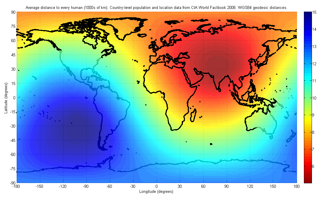
The geometric median is the point to which the population has the smallest possible sum of distances (or equivalently, the smallest average distance). Because of this property, it is also known as the point of minimum aggregate travel. Unfortunately, there is no direct closed-form expression for the geometric median; it is typically computed using iterative methods.[citation needed]

Determination

[edit]

In practical computation, decisions are also made on the granularity (coarseness) of the population data, depending on population density patterns or other factors. For instance, the center of population of all the cities in a country may be different from the center of population of all the states (or provinces, or other subdivisions) in the same country. Different methods may yield different results.

Practical uses for finding the center of population include locating possible sites for forward capitals, such as Brasília, Astana or Austin, and, along the same lines, to make tax collection easier. Practical selection of a new site for a capital is a complex problem that depends also on population density patterns and transportation networks.

World

[edit]

It is important to use a method that does not depend on a two-dimensional projection when dealing with the entire world. In a study from the Institut national d'études démographiques,[4] the solution methodology deals only with the globe. As a result, the answer is independent of which map projection is used or where it is centered. As described above, the exact location of the center of population will depend on both the granularity of the population data used, and the distance metric. With geodesic distances as the metric, and a granularity of 1,000 kilometers (600 mi), meaning that two population centers within 1000 km of each other are treated as part of a larger common population center of intermediate location, the world's center of population is found to lie "at the crossroads between China, India, Pakistan and Tajikistan" with an average distance of 5,200 kilometers (3,200 mi) to all humans.[4] The data used in the reference support this result to a precision of only a few hundred kilometers, hence the exact location is not known.

Another analysis, using city-level population data, found that the world's center of population is close to Almaty, Kazakhstan.[5]

By country

[edit]

Antigua and Barbuda

[edit]

In 2011, the center of population of Antigua (excluding Barbuda) was located in St. Claire.[6]

Australia

[edit]

Australia's population centroid is in central New South Wales. By 1996, it had moved only a little to the north-west since 1911.[7] It moved only 1.4 km north in 2022 from the previous year[8] and in 2023 moved 1.9 km west compared to 2022, located 40 km east of Ivanhoe.[9]

Canada

[edit]

In Canada, a 1986 study placed the point of minimum aggregate travel just north of Toronto in the city of Richmond Hill, and moving westward at a rate of approximately 2 meters per day.[10]

China

[edit]

China's population centroid has wandered within southern Henan from 1952 to 2005. Incidentally, the two end point dates are remarkably close to each other.[11] China also plots its economic centroid or center of economy/GDP, which has also wandered, and is generally located at the eastern Henan borders.[11]

Estonia

[edit]
European Countries median center of population in 2011

The center of population of Estonia was on the northwestern shore of Lake Võrtsjärv in 1913 and moved an average of 6 km northwest with every decade until the 1970s. The higher immigration rates during the late Soviet occupation to mostly Tallinn and Northeastern Estonia resulted the center of population moving faster towards north and continuing urbanization has seen it move northwest towards Tallinn since the 1990s. The center of population according to the 2011 census was in Jüri, just 6 km southeast from the border of Tallinn.[12]

Finland

[edit]

In Finland, the point of minimum aggregate travel is located in the former municipality of Hauho.[13] It is moving slightly to the south-west-west every year because people are moving out of the peripheral areas of northern and eastern Finland.

Germany

[edit]

In Germany, the centroid of the population is located in Spangenberg, Hesse, close to Kassel.[14]

Great Britain

[edit]

The centre of population in Great Britain did not move significantly in the 20th century. In 1901, it was in Rodsley, Derbyshire and in 1911 in Longford. In 1971 it was at Newhall, Swadlincote, South Derbyshire and in 2000, it was in Appleby Parva, Leicestershire.[15][16] Using the 2011 census the population centre can be calculated at Snarestone, Swadlincote.[17]

Ireland

[edit]

The center of population of the entire island of Ireland is located near Kilcock, County Kildare. This is significantly further east than the Geographical centre of Ireland, reflecting the disproportionately large cities of the east of the island (Belfast and Dublin).[18] The center of population of the Republic of Ireland is located southwest of Edenderry, County Offaly.[19]

Japan

[edit]

The centroid of population of Japan is in Gifu Prefecture, almost directly north of Nagoya city, and has been moving east-southeast for the past few decades.[20] Since 2010, the only large regions in Japan with significant population growth have been in Greater Tokyo and Okinawa Prefecture.

New Zealand

[edit]
New Zealand's median center of population over time

In June 2008, New Zealand's median center of population was located near Taharoa, around 100 km (65 mi) southwest of Hamilton on the North Island's west coast.[21] In 1900 it was near Nelson and has been moving steadily north (towards Auckland, the country's most populous city) ever since.[22]

Sweden

[edit]

The demographical center of Sweden (using the median center definition) is Hjortkvarn in Hallsberg Municipality, Örebro county. Between the 1989 and 2007 census the point moved a few kilometres to the south, due to a decreasing population in northern Sweden and immigration to the south.[23]

Russia

[edit]

The center of population in the Russian Federation is calculated by A. K. Gogolev to be at 56°26′N 53°04′E / 56.433°N 53.067°E / 56.433; 53.067 as of 2010, 46.5 km (28.9 mi) south-southwest of Izhevsk.[24]

Taiwan

[edit]

The center of population of Taiwan is located in Heping District, Taichung.[25]

United States

[edit]

The mean center of the United States population (using the centroid definition) has been calculated for each U.S. Census since 1790. Over the last two centuries, it has progressed westward and, since 1930, southwesterly, reflecting population drift. For example, in 2010, the mean center was located near Plato, Missouri, in the south-central part of the state, whereas, in 1790, it was in Kent County, Maryland, 47 miles (76 km) east-northeast of the future federal capital, Washington, D.C.

See also

[edit]

References

[edit]

Sources

[edit]
  • Bellone F. and Cunningham R. (1993). "All Roads Lead to... Laxton, Digby and Longford." Statistics Canada 1991 Census Short Articles Series.
[edit]
Revisions and contributorsEdit on WikipediaRead on Wikipedia
from Grokipedia
The center of population, also known as the population center, is a geographic point that represents the average location of a region's inhabitants, analogous to the center of mass in physics where each individual is treated as an equal weight placed on a flat . This concept identifies a balance point for the distribution, providing a single coordinate that summarizes where people live on average within a defined area such as a , state, or the . It serves as a key metric in and to track shifts in patterns over time. The most common type is the mean center of population, calculated using weighted averages of residential coordinates from census data at fine spatial scales, such as blocks or grid cells. For the (λ), it is the sum of ( at each × ) divided by the total ; for (φ), it adjusts for the Earth's by using the sum of ( × × cos()) divided by the sum of ( × cos()). An alternative is the median center, which locates the point where lines drawn north-south and east-west each split the exactly in half, making it less sensitive to outliers like clustered urban populations but more complex to compute iteratively. These methods rely on precise data from national censuses or global datasets, often projected onto flat surfaces for simplicity, though advanced computations account for . Centers of population are valuable for understanding demographic trends, , and , as their movement reveals patterns of migration, growth, and . For instance, , the mean center has shifted steadily westward and southward since 1790—from near , , to its 2020 position in —reflecting expansion, industrialization, and recent population booms in the and West. Similar calculations apply globally, with national centers often located near major population hubs; for example, many European ' centers lie in central urban areas due to concentrated settlement. Historically, these metrics have informed policy, such as placement, and continue to evolve with from and surveys.

Definitions

Mean center

The mean center of population is defined as the geographical point where an imaginary flat, weightless of a region would balance if weights equal to the number of inhabitants were placed at their respective locations, analogous to a or gravity for the distribution. This concept assumes a uniform on a planar surface, treating population as point masses to compute the average location. Mathematically, the mean center coordinates are calculated as the weighted arithmetic averages of the and of populated , where weights are the sizes. For ϕ\phi, it is given by: ϕˉ=i(piϕi)ipi\bar{\phi} = \frac{\sum_i (p_i \cdot \phi_i)}{\sum_i p_i} where pip_i is the at ii with ϕi\phi_i, and the sum is over all . Similarly for λ\lambda, the formula adjusts for the convergence of meridians: λˉ=i(piλicosϕi)i(picosϕi)\bar{\lambda} = \frac{\sum_i (p_i \cdot \lambda_i \cdot \cos \phi_i)}{\sum_i (p_i \cdot \cos \phi_i)} This yields the east-west coordinate, accounting for the in a simplified manner. To illustrate conceptually, consider a simple two-point distribution: one cluster of 100 people at coordinates (0°, 0°) and another of 200 people at (10°, 0°). The mean would lie at approximately (6.67°, 0°), the population-weighted average pulling toward the larger group. Such examples highlight how the mean center shifts proportionally with population imbalances. A key advantage of the mean center is its simplicity in computation, requiring only and division, while incorporating data from every individual or unit to reflect overall shifts accurately. However, it is highly sensitive to outliers, such as remote or sparsely populated areas with extreme coordinates, which can disproportionately influence the result. Among its limitations, the mean center assumes Euclidean distances on a flat plane, ignoring the Earth's and leading to distortions, particularly for east-west calculations in higher latitudes. Additionally, results are affected by map projections, as different projections (e.g., cylindrical equal-area versus sinusoidal) yield varying coordinates due to unequal area or distance preservation. In contrast to the median center, the mean center's sensitivity to extremes makes it less robust for skewed distributions.

Median center

The median center of population is defined as the geographic point formed by the intersection of the median latitude and the median longitude of a given population distribution. The median latitude is the line running east-west such that 50% of the population resides to the north and 50% to the south, while the median longitude is the line running north-south such that 50% of the population resides to the east and 50% to the west. To compute the median center, population data—typically from census records aggregated at county or smaller units—are sorted separately by latitude and longitude coordinates. For the median latitude, the units are ordered from south to north, and cumulative population is tallied until reaching the point where exactly half the total population lies on either side; the same process is applied independently for longitude from west to east. The resulting coordinates are then intersected to locate the median center. This axis-independent approach simplifies calculation compared to methods that integrate both dimensions simultaneously. For a hypothetical example in the , consider a population distributed across the contiguous states with major concentrations in urban areas like (northeast), Los Angeles (west coast), and (midwest). The latitude might fall near 38.30°N, balancing the dense populations of the Northeast and Midwest against sparser southern and western regions, such that approximately 165.7 million people (half of the 331.4 million total population as of the 2020 Census) live north of this line. Similarly, the longitude could be around 87.56°W, dividing the East Coast and Midwest densities from the less populated West, with half the population east of this meridian. The intersection would place the median center in Patoka Township, , illustrating how it captures balanced halves without being pulled toward distant outliers. One key advantage of the median center is its resistance to extreme population concentrations or outliers, making it suitable for skewed distributions where a small number of densely populated areas might otherwise distort the location. For instance, in regions with isolated megacities, the median center remains stable by focusing solely on population halves rather than weighted averages. Unlike the mean center, which can shift significantly due to such imbalances, the median provides a more robust measure of in unevenly distributed populations./03%3A_Examining_the_Evidence_Using_Graphs_and_Statistics/3.01%3A_Measures_of_Center A limitation of the median center is that it treats latitude and longitude axes independently, ignoring potential interactions between them in a two-dimensional geographic space. This can lead to a point that does not fully reflect the spatial cohesion of the population, particularly on curved surfaces like the where longitude lines converge at the poles.

Geometric median

The of a is the location that minimizes the sum of straight-line (Euclidean) distances to all individual population points, serving as a robust measure of in geographic and demographic analysis. This concept was formalized by in his seminal work on multivariate medians. Mathematically, for a set of nn locations xiR2x_i \in \mathbb{R}^2, i=1,,ni = 1, \dots, n, the p^\hat{p} is given by p^=argminpi=1npxi2,\hat{p} = \arg\min_p \sum_{i=1}^n \| p - x_i \|_2, where 2\| \cdot \|_2 denotes the Euclidean norm. Unlike the mean center, which simply averages coordinates, this formulation optimizes total distance but lacks a closed-form solution except in special cases, necessitating iterative numerical methods. A widely used approach is Weiszfeld's algorithm, an that approximates the optimum by successively weighting points inversely by their distances to the current estimate. A representative example is the geometric median for three non-collinear population points forming a triangle. If all interior angles are less than 120°, the median coincides with the Fermat-Torricelli point inside the triangle, from which line segments to the vertices subtend 120° angles, minimizing the total distance. If one angle is 120° or greater, the median locates at the vertex of that angle. The geometric median offers advantages in applications like facility location, where it identifies an optimal site (e.g., a distribution center) to minimize aggregate travel distances to population centers, providing robustness against outliers that could distort coordinate-based averages. However, its computation is intensive for large-scale datasets, often requiring O(n)O(n) operations per iteration and convergence monitoring, which scales poorly without approximations. Additionally, when applied to global or continental populations, the Euclidean metric assumes a flat plane and is sensitive to Earth's curvature; accurate modeling instead demands the Riemannian geometric median, minimizing sums of geodesic distances on the spherical manifold.

History

Origins and early uses

The concept of the center of population, analogous to the geometric centroid, has mathematical roots in ancient geometry. of Syracuse, in the 3rd century BCE, developed foundational theorems on the for plane figures, such as triangles and parabolas, treating it as the balance point where the figure could be supported without tipping. This idea influenced later statistical and geographic applications, though direct use for human populations emerged much later. In 19th-century , geographers like Karl Ritter advanced systematic studies of human-environment interactions, emphasizing regional population distributions in works such as Die Erdkunde (1817–1859), which indirectly paved the way for quantitative demographic centers by promoting comparative analysis of settlement patterns. In the United States, the center of population was formally introduced by Census Bureau officials in the 1870s as a tool to visualize national population trends and westward migration. The first official calculation appeared in the 1880 Census report, Statistics of the Population of the United States, where it was defined as the point on an imaginary flat map where the population would balance if represented by equal weights. Retrospective computations were soon applied to earlier censuses, including 1790, placing the initial mean center approximately 23 miles east of Baltimore in Kent County, Maryland—reflecting the heavy concentration of the young nation's 3.9 million people along the Atlantic seaboard. These early calculations highlighted dramatic shifts, such as the center moving about 40 miles westward by 1800 to a point 18 miles west of Baltimore in Howard County, Maryland, driven by frontier expansion into the Ohio Valley. The U.S. Census Bureau played a pivotal role in standardizing the method after the publication, incorporating it into subsequent decennial reports to monitor and growth patterns. For instance, the 1790–1880 series of centers traced a steady progression from the East Coast interior toward the Midwest, underscoring the impact of territorial acquisitions like the and railroad development. Prior to widespread adoption in national statistics, similar notions informed colonial administrative decisions; , in proposing a new capital for in 1776, argued for relocation based on the shifting "center of population" beyond the tidewater region to the Alleghenies, as Williamsburg had become outdated and vulnerable. Such pre-20th-century applications in colonial mapping and were qualitative and limited, often guiding the placement of seats of power in sparsely documented territories rather than precise computations.

Development in modern demography

In the 20th century, the calculation of population centers expanded beyond initial U.S. applications, becoming integrated into national census frameworks to track demographic shifts amid urbanization and industrialization. In the late 19th and early 20th centuries, the median center—which divides the population into equal halves along north-south and east-west lines—was introduced, offering a robust alternative to the mean center less sensitive to extreme distributions. Similarly, the geometric median emerged in statistical literature as a measure minimizing the sum of distances to all population points, particularly useful for non-Euclidean spaces and outlier-prone datasets. These variants addressed limitations in earlier arithmetic means, enabling more nuanced analyses of spatial population balance. Technological progress further revolutionized these computations starting in the , when manual tabulations gave way to computer-based processing using punched cards for data input and magnetic tapes for storage, allowing aggregation over thousands of small geographic units like enumeration districts. This shift improved precision by incorporating models and latitude corrections for east-west distances, reducing errors from flat-Earth assumptions. By the , the adoption of Geographic Information Systems (GIS) enabled geospatial analysis of centers, facilitating calculations with accurate distances and dynamic mapping of historical trends across counties or states. GIS tools, such as mean center functions in software like , weighted coordinates by to visualize shifts, supporting educational and research applications in . Global adoption of center analyses grew in the , with demographic institutions applying them to assess worldwide trends and inform policy. For instance, studies examined continental or global centers to understand migration's spatial impacts, integrating them into frameworks for urban and regional development. In , such metrics supported EU regional policies by highlighting population concentrations for and cohesion , emphasizing functional urban areas where centers indicate growth poles. Post-2010 developments have emphasized dynamic modeling to incorporate migration flows, projecting future centers under scenarios like climate-driven displacement that amplify urban-rural divides. These models couple cohort projections with multidimensional migration estimates, revealing how net movements alter spatial balances over decades. However, critiques persist regarding data granularity, especially in developing countries where irregular censuses and coarse gridded datasets underrepresent rural populations, leading to biased center estimates that overlook dispersed settlements. In policy contexts, population center calculations provide critical insights into distributional changes, influencing ; data, including population distribution metrics, inform the allocation of over $2.8 trillion in annual federal funding (as of 2021) for , and infrastructure programs responsive to demographic patterns.

Determination

Data sources and requirements

The calculation of a center of population requires primary demographic data in the form of population counts from censuses or equivalent surveys, typically aggregated at subnational administrative levels such as counties, municipalities, or smaller units like census blocks. These counts must be paired with precise geographic coordinates, usually latitude and longitude for each population unit's centroid, to enable weighted averaging. In the United States, for instance, the Census Bureau has utilized decennial census data since 1790, drawing on the TIGER database for coordinates of over 8 million block-level areas in the 2020 census computations. Data granularity varies from aggregated national or state-level summaries, which suffice for broad estimates but reduce precision, to highly disaggregated block- or grid-level distributions that enhance accuracy by capturing local variations. Finer improves the representational fidelity of population distribution but introduces trade-offs with privacy, as detailed microdata risks re-identification; modern mitigate this through techniques like , which add controlled noise to balance utility and protection. For example, the U.S. 2020 applied to block-level data, explicitly quantifying the privacy-accuracy trade-off via an parameter that limits disclosure risk while preserving aggregate statistics. Geographic adjustments are essential to account for the Earth's curvature, as simple Euclidean distances in - space distort east-west measurements at higher latitudes. Calculations often employ spherical approximations, such as scaling by the cosine of to approximate distances, rather than planar Euclidean methods, which are suitable only for small areas. Projection effects, like those in Mercator maps, must also be avoided by working directly in to prevent areal distortions that skew population weighting. Key data challenges include incomplete or outdated censuses, particularly in developing regions where coverage gaps persist due to logistical constraints and under-enumeration. The addresses these by integrating vital statistics—such as birth and death registrations—with sample surveys and model-based adjustments, estimating undercounts via post-enumeration surveys in over 320 instances. Migration effects are incorporated through cohort-component methods, using residuals from intercensal differences and administrative records to refine estimates where direct data is sparse. This approach has been pivotal in historical U.S. censuses for tracking internal shifts. Primary sources include national statistical bureaus, such as the U.S. Census Bureau for domestic data and the Australian Bureau of Statistics (ABS) for subnational census counts at Statistical Area Level 1. International organizations like the Population Division and the World Bank aggregate these for global estimates, compiling over 1,910 census datasets from 237 countries while filling gaps with probabilistic models.

Calculation methods and formulas

The calculation of a center of population generally involves weighting geographic coordinates by population sizes at discrete locations, such as census blocks or grid cells, to derive a representative point. For closed-form solutions like the mean center, this is a direct weighted average; for others, such as the , iterative algorithms are required to minimize the objective function due to the non-linear nature of distances. The center, analogous to the of a distribution, is computed as the population-weighted of coordinates. Assuming a set of nn locations with population pi>0p_i > 0 at coordinates (xi,yi)(x_i, y_i), where xix_i approximates and yiy_i , the center (xˉ,yˉ)(\bar{x}, \bar{y}) is given by: xˉ=i=1npixii=1npi,yˉ=i=1npiyii=1npi.\bar{x} = \frac{\sum_{i=1}^n p_i x_i}{\sum_{i=1}^n p_i}, \quad \bar{y} = \frac{\sum_{i=1}^n p_i y_i}{\sum_{i=1}^n p_i}. This derivation follows from minimizing the sum of squared distances pi(x,y)(xi,yi)2\sum p_i \| (x, y) - (x_i, y_i) \|^2, which yields the weighted as the minimizer. For applications on Earth's surface, the component is often adjusted to account for by incorporating the cosine of : xˉ=picosyixipicosyi\bar{x} = \frac{\sum p_i \cos y_i \cdot x_i}{\sum p_i \cos y_i}, reducing distortion at higher latitudes. The center is determined by finding the intersection of two lines that each divide the total in half along the north-south and east-west axes, providing a robust measure insensitive to extreme outliers. The steps are: (1) sort all locations by x-coordinate () and compute cumulative populations until reaching or exceeding 50% of the total P/2P/2, where P=piP = \sum p_i; select the location (or interpolate between two if the cumulative exactly hits P/2P/2) as the x-; (2) repeat for y-coordinates () to find the y-; (3) the center is the point at these medians. Ties, when the cumulative splits evenly between two adjacent , are handled by averaging their coordinates or selecting one based on convention, ensuring the division remains as balanced as possible. The minimizes the sum of weighted Euclidean (or great-circle) distances to all points, pi(x,y)(xi,yi)\sum p_i \| (x, y) - (x_i, y_i) \|, lacking a closed-form solution except in like collinear points. Weiszfeld's iterative , a fixed-point method, approximates it efficiently: initialize an estimate (x(0),y(0))(x^{(0)}, y^{(0)}) (e.g., the mean center); then iterate k=1,2,k = 1, 2, \dots until convergence: (x(k),y(k))=(i=1npi(xi,yi)(x(k1),y(k1))(xi,yi)i=1npi(x(k1),y(k1))(xi,yi)),(x^{(k)}, y^{(k)}) = \left( \frac{\sum_{i=1}^n \frac{p_i (x_i, y_i)}{\| (x^{(k-1)}, y^{(k-1)}) - (x_i, y_i) \| }}{\sum_{i=1}^n \frac{p_i}{\| (x^{(k-1)}, y^{(k-1)}) - (x_i, y_i) \| }} \right),
Add your contribution
Related Hubs
User Avatar
No comments yet.