Electromagnetic induction was discovered by Michael Faraday, published in 1831.^[3][4] It was discovered independently by Joseph Henry in 1832.^[5][6]

In Faraday's first experimental demonstration, on August 29, 1831,^[7] he wrapped two wires around opposite sides of an iron ring or "torus" (an arrangement similar to a modern toroidal transformer).^{[citation needed]} Based on his understanding of electromagnets, he expected that, when current started to flow in one wire, a sort of wave would travel through the ring and cause some electrical effect on the opposite side. He plugged one wire into a galvanometer, and watched it as he connected the other wire to a battery. He saw a transient current, which he called a "wave of electricity", when he connected the wire to the battery and another when he disconnected it.^[8] This induction was due to the change in magnetic flux that occurred when the battery was connected and disconnected.^[2] Within two months, Faraday found several other manifestations of electromagnetic induction. For example, he saw transient currents when he quickly slid a bar magnet in and out of a coil of wires, and he generated a steady (DC) current by rotating a copper disk near the bar magnet with a sliding electrical lead ("Faraday's disk").^[9]

Faraday explained electromagnetic induction using a concept he called lines of force. However, scientists at the time widely rejected his theoretical ideas, mainly because they were not formulated mathematically.^[10] An exception was James Clerk Maxwell, who used Faraday's ideas as the basis of his quantitative electromagnetic theory.^[10][11][12] In Maxwell's model, the time varying aspect of electromagnetic induction is expressed as a differential equation, which Oliver Heaviside referred to as Faraday's law even though it is slightly different from Faraday's original formulation and does not describe motional emf. Heaviside's version (see Maxwell–Faraday equation below) is the form recognized today in the group of equations known as Maxwell's equations.

In 1834 Heinrich Lenz formulated the law named after him to describe the "flux through the circuit". Lenz's law gives the direction of the induced emf and current resulting from electromagnetic induction.

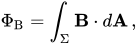
Faraday's law of induction makes use of the magnetic flux Φ_B through a region of space enclosed by a wire loop. The magnetic flux is defined by a surface integral:^[13] $${\displaystyle \Phi _{\mathrm {B} }=\int _{\Sigma }\mathbf {B} \cdot d\mathbf {A} \,,}$$ where dA is an element of the surface Σ enclosed by the wire loop, B is the magnetic field. The dot product B·dA corresponds to an infinitesimal amount of magnetic flux. In more visual terms, the magnetic flux through the wire loop is proportional to the number of magnetic field lines that pass through the loop.

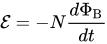
When the flux through the surface changes, Faraday's law of induction says that the wire loop acquires an electromotive force (emf).^{[note 1]} The most widespread version of this law states that the induced electromotive force in any closed circuit is equal to the rate of change of the magnetic flux enclosed by the circuit:^[17][18] $${\displaystyle {\mathcal {E}}=-{\frac {d\Phi _{\mathrm {B} }}{dt}}\,,}$$ where ${\displaystyle {\mathcal {E}}}$ is the emf and Φ_B is the magnetic flux. The direction of the electromotive force is given by Lenz's law which states that an induced current will flow in the direction that will oppose the change which produced it.^[19] This is due to the negative sign in the previous equation. To increase the generated emf, a common approach is to exploit flux linkage by creating a tightly wound coil of wire, composed of N identical turns, each with the same magnetic flux going through them. The resulting emf is then N times that of one single wire.^[20][21] $${\displaystyle {\mathcal {E}}=-N{\frac {d\Phi _{\mathrm {B} }}{dt}}}$$

Generating an emf through a variation of the magnetic flux through the surface of a wire loop can be achieved in several ways:

1. the magnetic field B changes (e.g. an alternating magnetic field, or moving a wire loop towards a bar magnet where the B field is stronger),
2. the wire loop is deformed and the surface Σ changes,
3. the orientation of the surface dA changes (e.g. spinning a wire loop into a fixed magnetic field),
4. any combination of the above

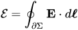
In general, the relation between the emf ${\displaystyle {\mathcal {E}}}$ in a wire loop encircling a surface Σ, and the electric field E in the wire is given by $${\displaystyle {\mathcal {E}}=\oint _{\partial \Sigma }\mathbf {E} \cdot d{\boldsymbol {\ell }}}$$ where dℓ is an element of contour of the surface Σ, combining this with the definition of flux $${\displaystyle \Phi _{\mathrm {B} }=\int _{\Sigma }\mathbf {B} \cdot d\mathbf {A} \,,}$$ we can write the integral form of the Maxwell–Faraday equation $${\displaystyle \oint _{\partial \Sigma }\mathbf {E} \cdot d{\boldsymbol {\ell }}=-{\frac {d}{dt}}{\int _{\Sigma }\mathbf {B} \cdot d\mathbf {A} }}$$

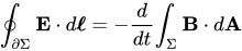
It is one of the four Maxwell's equations, and therefore plays a fundamental role in the theory of classical electromagnetism.

Faraday's law describes two different phenomena: the motional emf generated by a magnetic force on a moving wire (see Lorentz force), and the transformer emf that is generated by an electric force due to a changing magnetic field (due to the differential form of the Maxwell–Faraday equation). James Clerk Maxwell drew attention to the separate physical phenomena in 1861.^[22][23] This is believed to be a unique example in physics of where such a fundamental law is invoked to explain two such different phenomena.^[24]

Albert Einstein noticed that the two situations both corresponded to a relative movement between a conductor and a magnet, and the outcome was unaffected by which one was moving. This was one of the principal paths that led him to develop special relativity.^[25]

The principles of electromagnetic induction are applied in many devices and systems, including:

The emf generated by Faraday's law of induction due to relative movement of a circuit and a magnetic field is the phenomenon underlying electrical generators. When a permanent magnet is moved relative to a conductor, or vice versa, an electromotive force is created. If the wire is connected through an electrical load, current will flow, and thus electrical energy is generated, converting the mechanical energy of motion to electrical energy. For example, the drum generator is based upon the figure to the bottom-right. A different implementation of this idea is the Faraday's disc, shown in simplified form on the right.

In the Faraday's disc example, the disc is rotated in a uniform magnetic field perpendicular to the disc, causing a current to flow in the radial arm due to the Lorentz force. Mechanical work is necessary to drive this current. When the generated current flows through the conducting rim, a magnetic field is generated by this current through Ampère's circuital law (labelled "induced B" in the figure). The rim thus becomes an electromagnet that resists rotation of the disc (an example of Lenz's law). On the far side of the figure, the return current flows from the rotating arm through the far side of the rim to the bottom brush. The B-field induced by this return current opposes the applied B-field, tending to decrease the flux through that side of the circuit, opposing the increase in flux due to rotation. On the near side of the figure, the return current flows from the rotating arm through the near side of the rim to the bottom brush. The induced B-field increases the flux on this side of the circuit, opposing the decrease in flux due to r the rotation. The energy required to keep the disc moving, despite this reactive force, is exactly equal to the electrical energy generated (plus energy wasted due to friction, Joule heating, and other inefficiencies). This behavior is common to all generators converting mechanical energy to electrical energy.

When the electric current in a loop of wire changes, the changing current creates a changing magnetic field. A second wire in reach of this magnetic field will experience this change in magnetic field as a change in its coupled magnetic flux, ${\displaystyle {\frac {d\Phi _{B}}{dt}}}$. Therefore, an electromotive force is set up in the second loop called the induced emf or transformer emf. If the two ends of this loop are connected through an electrical load, current will flow.

A current clamp is a type of transformer with a split core which can be spread apart and clipped onto a wire or coil to either measure the current in it or, in reverse, to induce a voltage. Unlike conventional instruments the clamp does not make electrical contact with the conductor or require it to be disconnected during attachment of the clamp.

Faraday's law is used for measuring the flow of electrically conductive liquids and slurries. Such instruments are called magnetic flow meters. The induced voltage ε generated in the magnetic field B due to a conductive liquid moving at velocity v is thus given by:

${\displaystyle {\mathcal {E}}=-B\ell v,}$

where ℓ is the distance between electrodes in the magnetic flow meter.

Electrical conductors moving through a steady magnetic field, or stationary conductors within a changing magnetic field, will have circular currents induced within them by induction, called eddy currents. Eddy currents flow in closed loops in planes perpendicular to the magnetic field. They have useful applications in eddy current brakes and induction heating systems. However eddy currents induced in the metal magnetic cores of transformers and AC motors and generators are undesirable since they dissipate energy (called core losses) as heat in the resistance of the metal. Cores for these devices use a number of methods to reduce eddy currents:

• Cores of low frequency alternating current electromagnets and transformers, instead of being solid metal, are often made of stacks of metal sheets, called laminations, separated by nonconductive coatings. These thin plates reduce the undesirable parasitic eddy currents, as described below.
• Inductors and transformers used at higher frequencies often have magnetic cores made of nonconductive magnetic materials such as ferrite or iron powder held together with a resin binder.

Eddy currents occur when a solid metallic mass is rotated in a magnetic field, because the outer portion of the metal cuts more magnetic lines of force than the inner portion; hence the induced electromotive force is not uniform; this tends to cause electric currents between the points of greatest and least potential. Eddy currents consume a considerable amount of energy and often cause a harmful rise in temperature.^[26]

Only five laminations or plates are shown in this example, so as to show the subdivision of the eddy currents. In practical use, the number of laminations or punchings ranges from 40 to 66 per inch (16 to 26 per centimetre), and brings the eddy current loss down to about one percent. While the plates can be separated by insulation, the voltage is so low that the natural rust/oxide coating of the plates is enough to prevent current flow across the laminations.^[26]

This is a rotor approximately 20 mm in diameter from a DC motor used in a CD player. Note the laminations of the electromagnet pole pieces, used to limit parasitic inductive losses.

In this illustration, a solid copper bar conductor on a rotating armature is just passing under the tip of the pole piece N of the field magnet. Note the uneven distribution of the lines of force across the copper bar. The magnetic field is more concentrated and thus stronger on the left edge of the copper bar (a,b) while the field is weaker on the right edge (c,d). Since the two edges of the bar move with the same velocity, this difference in field strength across the bar creates whorls or current eddies within the copper bar.^[26]

High current power-frequency devices, such as electric motors, generators and transformers, use multiple small conductors in parallel to break up the eddy flows that can form within large solid conductors. The same principle is applied to transformers used at higher than power frequency, for example, those used in switch-mode power supplies and the intermediate frequency coupling transformers of radio receivers.

Electromagnetism
Electricity Magnetism Optics History Computational Textbooks Phenomena
Electrostatics Charge density Conductor Coulomb law Electret Electric charge Electric dipole Electric field Electric flux Electric potential Electrostatic discharge Electrostatic induction Gauss's law Insulator Permittivity Polarization Potential energy Static electricity Triboelectricity
Magnetostatics Ampère's law Biot–Savart law Gauss's law for magnetism Magnetic dipole Magnetic field Magnetic flux Magnetic scalar potential Magnetic vector potential Magnetization Permeability Right-hand rule
Electrodynamics Bremsstrahlung Cyclotron radiation Displacement current Eddy current Electromagnetic field Electromagnetic induction Electromagnetic pulse Electromagnetic radiation Faraday's law Jefimenko equations Larmor formula Lenz's law Liénard–Wiechert potential London equations Lorentz force Maxwell's equations Maxwell tensor Poynting vector Synchrotron radiation
Electrical network Alternating current Capacitance Current density Direct current Electric current Electric power Electrolysis Electromotive force Impedance Inductance Joule heating Kirchhoff's laws Network analysis Ohm's law Parallel circuit Resistance Resonant cavities Series circuit Voltage Watt Waveguides
Magnetic circuit AC motor DC motor Electric machine Electric motor Gyrator–capacitor Induction motor Linear motor Magnetomotive force Permeance Reluctance (complex) Reluctance (real) Rotor Stator Transformer
Covariant formulation Electromagnetic tensor Electromagnetism and special relativity Four-current Four-potential Mathematical descriptions Maxwell equations in curved spacetime Relativistic electromagnetism Stress–energy tensor
Scientists Ampère Biot Coulomb Davy Einstein Faraday Fizeau Gauss Heaviside Helmholtz Henry Hertz Hopkinson Jefimenko Joule Kelvin Kirchhoff Larmor Lenz Liénard Lorentz Maxwell Neumann Ohm Ørsted Poisson Poynting Ritchie Savart Singer Steinmetz Tesla Thomson Volta Weber Wiechert
v t e

• Alternator – Device converting mechanical into electrical energy
• Crosstalk – Signals in one channel affecting another
• Faraday paradox – Apparent paradox with Faraday's law of induction
• Fleming's right-hand rule – Mnemonic for the direction of induced current in a moving magnetic field
• Hall effect – Electromagnetic effect in physics
• Inductance
• Moving magnet and conductor problem