
Solar phenomena
View on WikipediaThis article has multiple issues. Please help improve it or discuss these issues on the talk page. (Learn how and when to remove these messages)
|

Solar phenomena are natural phenomena which occur within the atmosphere of the Sun. They take many forms, including solar wind, radio wave flux, solar flares, coronal mass ejections,[1] coronal heating and sunspots.
These phenomena are believed to be generated by a helical dynamo, located near the center of the Sun's mass, which generates strong magnetic fields, as well as a chaotic dynamo, located near the surface, which generates smaller magnetic field fluctuations.[2] All solar fluctuations together are referred to as solar variation, producing space weather within the Sun's gravitational field.
Solar activity and related events have been recorded since the eighth century BCE. Throughout history, observation technology and methodology advanced, and in the 20th century, interest in astrophysics surged and many solar telescopes were constructed. The 1931 invention of the coronagraph allowed the corona to be studied in full daylight.
Sun
[edit]
The Sun is a star located at the center of the Solar System. It is almost perfectly spherical and consists of hot plasma and magnetic fields.[3][4] It has a diameter of about 1,392,684 kilometres (865,374 mi),[5] around 109 times that of Earth, and its mass (1.989×1030 kilograms, approximately 330,000 times that of Earth) accounts for some 99.86% of the total mass of the Solar System.[6] Chemically, about three quarters of the Sun's mass consists of hydrogen, while the rest is mostly helium. The remaining 1.69% (equal to 5,600 times the mass of Earth) consists of heavier elements, including oxygen, carbon, neon and iron.[7]
The Sun formed about 4.567 billion[a][8] years ago from the gravitational collapse of a region within a large molecular cloud. Most of the matter gathered in the center, while the rest flattened into an orbiting disk that became the balance of the Solar System. The central mass became increasingly hot and dense, eventually initiating thermonuclear fusion in its core.
The Sun is a G-type main-sequence star (G2V) based on spectral class, and it is informally designated as a yellow dwarf because its visible radiation is most intense in the yellow-green portion of the spectrum. It is actually white, but from the Earth's surface, it appears yellow because of atmospheric scattering of blue light.[9] In the spectral class label, G2 indicates its surface temperature, of approximately 5770 K [3] ( the UAI will accept in 2014 5772 K ) and V indicates that the Sun, like most stars, is a main-sequence star, and thus generates its energy via fusing hydrogen into helium. In its core, the Sun fuses about 620 million metric tons of hydrogen each second.[10][11]
The Earth's mean distance from the Sun is approximately 1 astronomical unit (about 150,000,000 km; 93,000,000 mi), though the distance varies as the Earth moves from perihelion in January to aphelion in July.[12] At this average distance, light travels from the Sun to Earth in about 8 minutes, 19 seconds. The energy of this sunlight supports almost all life[b] on Earth by photosynthesis,[13] and drives Earth's climate and weather.[14] As recent as the 19th century, scientists had little knowledge of the Sun's physical composition and source of energy. This understanding is still developing; a number of present-day anomalies in the Sun's behavior remain unexplained.
Solar cycle
[edit]
Many solar phenomena change periodically over an average interval of about 11 years. This solar cycle affects solar irradiation and influences space weather, terrestrial weather, and climate.
The solar cycle also modulates the flux of short-wavelength solar radiation, from ultraviolet to X-ray and influences the frequency of solar flares, coronal mass ejections and other solar eruptive phenomena.
Types
[edit]| Part of a series of articles about |
| Heliophysics |
|---|
 |
Coronal mass ejections
[edit]A coronal mass ejection (CME) is a massive burst of solar wind and magnetic fields rising above the solar corona.[15] Near solar maxima, the Sun produces about three CMEs every day, whereas solar minima feature about one every five days.[16] CMEs, along with solar flares of other origin, can disrupt radio transmissions and damage satellites and electrical transmission line facilities, resulting in potentially massive and long-lasting power outages.[17][18]
Coronal mass ejections often appear with other forms of solar activity, most notably solar flares, but no causal relationship has been established. Most weak flares do not have CMEs; however, most powerful ones do. Most ejections originate from active regions on the Sun's surface, such as sunspot groupings associated with frequent flares. Other forms of solar activity frequently associated with coronal mass ejections are eruptive prominences, coronal dimming, coronal waves and Moreton waves, also called solar tsunami.
Magnetic reconnection is responsible for CME and solar flares. Magnetic reconnection is the name given to the rearrangement of magnetic field lines when two oppositely directed magnetic fields are brought together. This rearrangement is accompanied with a sudden release of energy stored in the original oppositely directed fields.[19][20]
When a CME impacts the Earth's magnetosphere, it temporarily deforms the Earth's magnetic field, changing the direction of compass needles and inducing large electrical ground currents in Earth itself; this is called a geomagnetic storm, and it is a global phenomenon. CME impacts can induce magnetic reconnection in Earth's magnetotail (the midnight side of the magnetosphere); this launches protons and electrons downward toward Earth's atmosphere, where they form the aurora.
Flares
[edit]A solar flare is a sudden flash of brightness observed over the Sun's surface or the solar limb, which is interpreted as an energy release of up to 6 × 1025 joules (about a sixth of the total Sun's energy output each second or 160 billion megatons of TNT equivalent, over 25,000 times more energy than released from the impact of Comet Shoemaker–Levy 9 with Jupiter). It may be followed by a coronal mass ejection.[21] The flare ejects clouds of electrons, ions and atoms through the corona into space. These clouds typically reach Earth a day or two after the event.[22] Similar phenomena in other stars are known as stellar flares.
Solar flares strongly influence space weather near the Earth. They can produce streams of highly energetic particles in the solar wind, known as a solar proton event. These particles can impact the Earth's magnetosphere in the form of a geomagnetic storm and present radiation hazards to spacecraft and astronauts.
- A solar flare
-
 On August 31, 2012, a long prominence/filament of solar material that had been hovering in the Sun's atmosphere, the corona, erupted out into space at 4:36 p.m. EDT.
 -
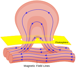 Diagram of the magnetic-field structure of a solar flare and its origin, inferred to result from the deformation of such a magnetic structure linking the solar interior with the solar atmosphere up through the corona.
 -
 A complete 2D-Image taken by STEREO (High Resolution)


Solar proton events
[edit]
A solar proton event (SPE), or "proton storm", occurs when particles (mostly protons) emitted by the Sun become accelerated either close to the Sun during a flare or in interplanetary space by CME shocks. The events can include other nuclei such as helium ions and HZE ions. These particles cause multiple effects. They can penetrate the Earth's magnetic field and cause ionization in the ionosphere. The effect is similar to auroral events, except that protons rather than electrons are involved. Energetic protons are a significant radiation hazard to spacecraft and astronauts.[23] Energetic protons can reach Earth within 30 minutes of a major flare's peak.
Prominences
[edit]A prominence is a large, bright, gaseous feature extending outward from the Sun's surface, often in the shape of a loop. Prominences are anchored to the Sun's surface in the photosphere and extend outwards into the corona. While the corona consists of high temperature plasma, which does not emit much visible light, prominences contain much cooler plasma, similar in composition to that of the chromosphere.
Prominence plasma is typically a hundred times cooler and denser than coronal plasma. A prominence forms over timescales of about an earthly day and may persist for weeks or months. Some prominences break apart and form CMEs.
A typical prominence extends over many thousands of kilometers; the largest on record was estimated at over 800,000 kilometres (500,000 mi) long [24] – roughly the solar radius.
When a prominence is viewed against the Sun instead of space, it appears darker than the background. This formation is called a solar filament.[24] It is possible for a projection to be both a filament and a prominence. Some prominences are so powerful that they eject matter at speeds ranging from 600 km/s to more than 1000 km/s. Other prominences form huge loops or arching columns of glowing gases over sunspots that can reach heights of hundreds of thousands of kilometers.[25]
Sunspots
[edit]Sunspots are relatively dark areas on the Sun's radiating 'surface' (photosphere) where intense magnetic activity inhibits convection and cools the Photosphere. Faculae are slightly brighter areas that form around sunspot groups as the flow of energy to the photosphere is re-established and both the normal flow and the sunspot-blocked energy elevate the radiating 'surface' temperature. Scientists began speculating on possible relationships between sunspots and solar luminosity in the 17th century.[26][27] Luminosity decreases caused by sunspots (generally < - 0.3%) are correlated with increases (generally < + 0.05%) caused both by faculae that are associated with active regions as well as the magnetically active 'bright network'.[28]
The net effect during periods of enhanced solar magnetic activity is increased radiant solar output because faculae are larger and persist longer than sunspots. Conversely, periods of lower solar magnetic activity and fewer sunspots (such as the Maunder Minimum) may correlate with times of lower irradiance.[29]
Sunspot activity has been measured using the Wolf number for about 300 years. This index (also known as the Zürich number) uses both the number of sunspots and the number of sunspot groups to compensate for measurement variations. A 2003 study found that sunspots had been more frequent since the 1940s than in the previous 1150 years.[30]
Sunspots usually appear as pairs with opposite magnetic polarity.[31] Detailed observations reveal patterns, in yearly minima and maxima and in relative location. As each cycle proceeds, the latitude of spots declines, from 30 to 45° to around 7° after the solar maximum. This latitudinal change follows Spörer's law.
For a sunspot to be visible to the human eye it must be about 50,000 km in diameter, covering 2,000,000,000 square kilometres (770,000,000 sq mi) or 700 millionths of the visible area. Over recent cycles, approximately 100 sunspots or compact sunspot groups are visible from Earth.[c][32]
Sunspots expand and contract as they move about and can travel at a few hundred meters per second when they first appear.
-
 Spörer's law noted that at the start of an 11-year sunspot cycle, the spots appeared first at higher latitudes and later in progressively lower latitudes.
 -
 A report in the Daily Mail characterized sunspot 1302 as a "behemoth" unleashing huge solar flares.
 -
 Detail of the Sun's surface, analog photography with a 4" Refractor, yellow glass filter and foil filter ND 4, Observatory Großhadern, Munich
 -
 Detailed view of sunspot, 13 December 2006


Wind
[edit]

The solar wind is a stream of plasma released from the Sun's upper atmosphere. It consists of mostly electrons and protons with energies usually between 1.5 and 10 keV. The stream of particles varies in density, temperature and speed over time and over solar longitude. These particles can escape the Sun's gravity because of their high energy.
The solar wind is divided into the slow solar wind and the fast solar wind. The slow solar wind has a velocity of about 400 kilometres per second (250 mi/s), a temperature of 2×10⁵ K and a composition that is a close match to the corona. The fast solar wind has a typical velocity of 750 km/s, a temperature of 8×10⁵ K and nearly matches the photosphere's.[33][34] The slow solar wind is twice as dense and more variable in intensity than the fast solar wind. The slow wind has a more complex structure, with turbulent regions and large-scale organization.[35][36]
Both the fast and slow solar winds can be interrupted by large, fast-moving bursts of plasma called interplanetary CMEs, or ICMEs. They cause shock waves in the thin plasma of the heliosphere, generating electromagnetic waves and accelerating particles (mostly protons and electrons) to form showers of ionizing radiation that precede the CME.
Effects
[edit]Space weather
[edit]
Space weather is the environmental condition within the Solar System, including the solar wind. It is studied especially surrounding the Earth, including conditions from the magnetosphere to the ionosphere and thermosphere. Space weather is distinct from terrestrial weather of the troposphere and stratosphere. The term was not used until the 1990s. Prior to that time, such phenomena were considered to be part of physics or aeronomy.
Solar storms
[edit]Solar storms are caused by disturbances on the Sun, most often coronal clouds associated with solar flare CMEs emanating from active sunspot regions, or less often from coronal holes. The Sun can produce intense geomagnetic and proton storms capable of causing power outages, disruption or communications blackouts (including GPS systems) and temporary/permanent disabling of satellites and other spaceborne technology. Solar storms may be hazardous to high-latitude, high-altitude aviation and to human spaceflight.[37] Geomagnetic storms cause aurorae.[38]
The most significant known solar storm occurred in September 1859 and is known as the Carrington event.[39][40]
Aurora
[edit]An aurora is a natural light display in the sky, especially in the high latitude (Arctic and Antarctic) regions, in the form of a large circle around the pole. It is caused by the collision of solar wind and charged magnetospheric particles with the high altitude atmosphere (thermosphere).
Most auroras occur in a band known as the auroral zone,[41][42] which is typically 3° to 6° wide in latitude and observed at 10° to 20° from the geomagnetic poles at all longitudes, but often most vividly around the spring and autumn equinoxes. The charged particles and solar wind are directed into the atmosphere by the Earth's magnetosphere. A geomagnetic storm expands the auroral zone to lower latitudes.
Auroras are associated with the solar wind. The Earth's magnetic field traps its particles, many of which travel toward the poles where they are accelerated toward Earth. Collisions between these ions and the atmosphere release energy in the form of auroras appearing in large circles around the poles. Auroras are more frequent and brighter during the solar cycle's intense phase when CMEs increase the intensity of the solar wind.[43]
Geomagnetic storm
[edit]A geomagnetic storm is a temporary disturbance of the Earth's magnetosphere caused by a solar wind shock wave and/or cloud of magnetic field that interacts with the Earth's magnetic field. The increase in solar wind pressure compresses the magnetosphere and the solar wind's magnetic field interacts with the Earth's magnetic field to transfer increased energy into the magnetosphere. Both interactions increase plasma movement through the magnetosphere (driven by increased electric fields) and increase the electric current in the magnetosphere and ionosphere.[44]
The disturbance in the interplanetary medium that drives a storm may be due to a CME or a high speed stream (co-rotating interaction region or CIR)[45] of the solar wind originating from a region of weak magnetic field on the solar surface. The frequency of geomagnetic storms increases and decreases with the sunspot cycle. CME driven storms are more common during the solar maximum of the solar cycle, while CIR-driven storms are more common during the solar minimum.
Several space weather phenomena are associated with geomagnetic storms. These include Solar Energetic Particle (SEP) events, geomagnetically induced currents (GIC), ionospheric disturbances that cause radio and radar scintillation, disruption of compass navigation and auroral displays at much lower latitudes than normal. A 1989 geomagnetic storm energized ground induced currents that disrupted electric power distribution throughout most of the province of Quebec[46] and caused aurorae as far south as Texas.[47]
Sudden ionospheric disturbance
[edit]A sudden ionospheric disturbance (SID) is an abnormally high ionization/plasma density in the D region of the ionosphere caused by a solar flare. The SID results in a sudden increase in radio-wave absorption that is most severe in the upper medium frequency (MF) and lower high frequency (HF) ranges, and as a result, often interrupts or interferes with telecommunications systems.[48]
Geomagnetically induced currents
[edit]Geomagnetically induced currents are a manifestation at ground level of space weather, which affect the normal operation of long electrical conductor systems. During space weather events, electric currents in the magnetosphere and ionosphere experience large variations, which manifest also in the Earth's magnetic field. These variations induce currents (GIC) in earthly conductors. Electric transmission grids and buried pipelines are common examples of such conductor systems. GIC can cause problems such as increased corrosion of pipeline steel and damaged high-voltage power transformers.
Carbon-14
[edit]
The production of carbon-14 (radiocarbon: 14C) is related to solar activity. Carbon-14 is produced in the upper atmosphere when cosmic ray bombardment of atmospheric nitrogen (14N) induces the nitrogen to undergo β+ decay, thus transforming into an unusual isotope of carbon with an atomic weight of 14 rather than the more common 12. Because galactic cosmic rays are partially excluded from the Solar System by the outward sweep of magnetic fields in the solar wind, increased solar activity reduces 14C production.[49]
Atmospheric 14C concentration is lower during solar maxima and higher during solar minima. By measuring the captured 14C in wood and counting tree rings, production of radiocarbon relative to recent wood can be measured and dated. A reconstruction of the past 10,000 years shows that the 14C production was much higher during the mid-Holocene 7,000 years ago and decreased until 1,000 years ago. In addition to variations in solar activity, long-term trends in carbon-14 production are influenced by changes in the Earth's geomagnetic field and by changes in carbon cycling within the biosphere (particularly those associated with changes in the extent of vegetation between ice ages).[citation needed]
Observation history
[edit]Solar activity and related events have been regularly recorded since the time of the Babylonians. Early records described solar eclipses, the corona and sunspots.

Soon after the invention of telescopes, in the early 1600s, astronomers began observing the Sun. Thomas Harriot was the first to observe sunspots, in 1610. Observers confirmed the less-frequent sunspots and aurorae during the Maunder minimum.[50] One of these observers was the renowned astronomer Johannes Hevelius who recorded a number of sunspots from 1653 to 1679 in the early Maunder minimum, listed in the book Machina Coelestis (1679).[51]
Solar spectrometry began in 1817.[52] Rudolf Wolf gathered sunspot observations as far back as the 1755–1766 cycle. He established a relative sunspot number formulation (the Wolf or Zürich sunspot number) that became the standard measure. Around 1852, Sabine, Wolf, Gautier and von Lamont independently found a link between the solar cycle and geomagnetic activity.[52]
On 2 April 1845, Fizeau and Foucault first photographed the Sun. Photography assisted in the study of solar prominences, granulation, spectroscopy and solar eclipses.[52]
On 1 September 1859, Richard C. Carrington and separately R. Hodgson first observed a solar flare.[52] Carrington and Gustav Spörer discovered that the Sun exhibits differential rotation, and that the outer layer must be fluid.[52]
In 1907–08, George Ellery Hale uncovered the Sun's magnetic cycle and the magnetic nature of sunspots. Hale and his colleagues later deduced Hale's polarity laws that described its magnetic field.[52]
Bernard Lyot's 1931 invention of the coronagraph allowed the corona to be studied in full daylight.[52]
The Sun was, until the 1990s, the only star whose surface had been resolved.[53] Other major achievements included understanding of:[54]
- X-ray-emitting loops (e.g., by Yohkoh)
- Corona and solar wind (e.g., by SoHO)
- Variance of solar brightness with level of activity, and verification of this effect in other solar-type stars (e.g., by ACRIM)
- The intense fibril state of the magnetic fields at the visible surface of a star like the Sun (e.g., by Hinode)
- The presence of magnetic fields of 0.5×10⁵ to 1×10⁵ gauss at the base of the conductive zone, presumably in some fibril form, inferred from the dynamics of rising azimuthal flux bundles.
- Low-level electron neutrino emission from the Sun's core.[54]
In the later twentieth century, satellites began observing the Sun, providing many insights. For example, modulation of solar luminosity by magnetically active regions was confirmed by satellite measurements of total solar irradiance (TSI) by the ACRIM1 experiment on the Solar Maximum Mission (launched in 1980).[28]
See also
[edit]Notes
[edit]- ^ All numbers in this article are short scale. One billion is 109, or 1,000,000,000.
- ^ Hydrothermal vent communities live so deep under the sea that they have no access to sunlight. Bacteria instead use sulfur compounds as an energy source, via chemosynthesis.
- ^ This is based on the hypothesis that the average human eye may have a resolution of 3.3×10⁻⁴ radians or 70 arc seconds, with a 1.5 millimetres (0.059 in) maximum pupil dilation in relatively bright light.[32]
References
[edit]- ^ Siscoe, George L.; Schrijver, Carolus J., eds. (2010). Heliophysics: evolving solar activity and the climates of space and earth (1. publ. ed.). Cambridge: Cambridge University Press. ISBN 978-0-521-11294-9. Retrieved 28 August 2014.
- ^ Giampapa, Mark S; Hill, Frank; Norton, Aimee A; Pevtsov, Alexei A. "Causes of Solar Activity" (PDF). A Science White Paper for the Heliophysics 2010 Decadal Survey: 1. Retrieved 26 August 2014.
- ^ "How Round is the Sun?". NASA. 2 October 2008. Archived from the original on 17 September 2018. Retrieved 7 March 2011.
- ^ "First Ever STEREO Images of the Entire Sun". NASA. 6 February 2011. Archived from the original on 8 March 2011. Retrieved 7 March 2011.
- ^ Emilio, M.; Kuhn, J. R.; Bush, R. I.; Scholl, I. F. (2012). "Measuring the Solar Radius from Space during the 2003 and 2006 Mercury Transits". The Astrophysical Journal. 750 (2): 135. arXiv:1203.4898. Bibcode:2012ApJ...750..135E. doi:10.1088/0004-637X/750/2/135. S2CID 119255559.
- ^ Woolfson, M. (2000). "The origin and evolution of the solar system". Astronomy & Geophysics. 41 (1): 1.12 – 1.19. Bibcode:2000A&G....41a..12W. CiteSeerX 10.1.1.475.5365. doi:10.1046/j.1468-4004.2000.00012.x.
- ^ Basu, S.; Antia, H. M. (2008). "Helioseismology and Solar Abundances". Physics Reports. 457 (5–6): 217–283. arXiv:0711.4590. Bibcode:2008PhR...457..217B. doi:10.1016/j.physrep.2007.12.002. S2CID 119302796.
- ^ Connelly, James N.; Bizzarro, Martin; Krot, Alexander N.; Nordlund, Åke; Wielandt, Daniel; Ivanova, Marina A. (2 November 2012). "The Absolute Chronology and Thermal Processing of Solids in the Solar Protoplanetary Disk". Science. 338 (6107): 651–655. Bibcode:2012Sci...338..651C. doi:10.1126/science.1226919. PMID 23118187. S2CID 21965292.
- ^ Wilk, S. R. (2009). "The Yellow Sun Paradox". Optics & Photonics News: 12–13. Archived from the original on 2012-06-18.
- ^ Phillips, K. J. H. (1995). Guide to the Sun. Cambridge University Press. pp. 47–53. ISBN 978-0-521-39788-9.
- ^ Kruszelnicki, Karl S. (17 April 2012). "Dr Karl's Great Moments In Science: Lazy Sun is less energetic than compost". Australian Broadcasting Corporation. Retrieved 25 February 2014.
Every second, the Sun burns 620 million tonnes of hydrogen...
- ^ "Equinoxes, Solstices, Perihelion, and Aphelion, 2000–2020". US Naval Observatory. 31 January 2008. Archived from the original on 13 October 2007. Retrieved 17 July 2009.
- ^ Simon, A. (2001). The Real Science Behind the X-Files: Microbes, meteorites, and mutants. Simon & Schuster. pp. 25–27. ISBN 978-0-684-85618-6.
- ^ Portman, D. J. (1952-03-01). "Review of Cycles in Weather and Solar Activity. by Maxwell O. Johnson". The Quarterly Review of Biology. 27 (1): 136–137. doi:10.1086/398866. JSTOR 2812845.
- ^ Christian, Eric R. (5 March 2012). "Coronal Mass Ejections". NASA.gov. Archived from the original on 10 April 2000. Retrieved 9 July 2013.
- ^ Nicky Fox. "Coronal Mass Ejections". Goddard Space Flight Center @ NASA. Retrieved 2011-04-06.
- ^ Baker, Daniel N.; et al. (2008). Severe Space Weather Events – Understanding Societal and Economic Impacts: A Workshop Report. National Academies Press. p. 77. ISBN 978-0-309-12769-1.
- ^ Wired world is increasingly vulnerable to coronal ejections from the Sun, Aviation Week & Space Technology, 14 January 2013 issue, pp. 49–50: "But the most serious potential for damage rests with the transformers that maintain the proper voltage for efficient transmission of electricity through the grid."
- ^ "Coronal Mass Ejections: Scientists Unlock the Secrets of Exploding Plasma Clouds On the Sun". Science Daily.
- ^ [1] Archived 2021-02-24 at the Wayback Machine NASA Science
- ^ Kopp, G.; Lawrence, G; Rottman, G. (2005). "The Total Irradiance Monitor (TIM): Science Results". Solar Physics. 20 (1–2): 129–139. Bibcode:2005SoPh..230..129K. doi:10.1007/s11207-005-7433-9. S2CID 44013218.
- ^ Menzel, Whipple, and de Vaucouleurs, "Survey of the Universe", 1970
- ^ Contribution of High Charge and Energy (HZE) Ions During Solar-Particle Event of September 29, 1989 Kim, Myung-Hee Y.; Wilson, John W.; Cucinotta, Francis A.; Simonsen, Lisa C.; Atwell, William; Badavi, Francis F.; Miller, Jack, NASA Johnson Space Center; Langley Research Center, May 1999.
- ^ a b Atkinson, Nancy (August 6, 2012). "Huge Solar Filament Stretches Across the Sun". Universe Today. Retrieved August 11, 2012.
- ^ "About Filaments and Prominences". Retrieved 2010-01-02.
- ^ Eddy, J.A. (1990). "Samuel P. Langley (1834–1906)". Journal for the History of Astronomy. 21: 111–20. Bibcode:1990JHA....21..111E. doi:10.1177/002182869002100113. S2CID 118962423. Archived from the original on May 10, 2009.
- ^ Foukal, P. V.; Mack, P. E.; Vernazza, J. E. (1977). "The effect of sunspots and faculae on the solar constant". The Astrophysical Journal. 215: 952. Bibcode:1977ApJ...215..952F. doi:10.1086/155431.
- ^ a b Willson RC, Gulkis S, Janssen M, Hudson HS, Chapman GA (February 1981). "Observations of Solar Irradiance Variability". Science. 211 (4483): 700–2. Bibcode:1981Sci...211..700W. doi:10.1126/science.211.4483.700. PMID 17776650.
- ^ Rodney Viereck, NOAA Space Environment Center. The Sun-Climate Connection
- ^ Usoskin, Ilya G.; Solanki, Sami K.; Schüssler, Manfred; Mursula, Kalevi; Alanko, Katja (2003). "A Millennium Scale Sunspot Number Reconstruction: Evidence For an Unusually Active Sun Since the 1940s". Physical Review Letters. 91 (21) 211101. arXiv:astro-ph/0310823. Bibcode:2003PhRvL..91u1101U. doi:10.1103/PhysRevLett.91.211101. PMID 14683287. S2CID 20754479.
- ^ "Sunspots". NOAA. Retrieved 22 February 2013.
- ^ a b Kennwell, John (2014). "Naked Eye Sunspots". Bureau of Meteorology. Commonwealth of Australia. Archived from the original on 3 September 2014. Retrieved 29 August 2014.
- ^ Bruno, Roberto; Carbone, Vincenzo (2016). Turbulence in the Solar Wind. Switzerland: Springer International Publishing. p. 4. ISBN 978-3-319-43440-7.
- ^ Feldman, U.; Landi, E.; Schwadron, N. A. (2005). "On the sources of fast and slow solar wind". Journal of Geophysical Research. 110 (A7): A07109.1–A07109.12. Bibcode:2005JGRA..110.7109F. doi:10.1029/2004JA010918.
- ^ Kallenrode, May-Britt (2004). Space Physics: An Introduction to Plasmas and. Springer. ISBN 978-3-540-20617-0.
- ^ Suess, Steve (June 3, 1999). "Overview and Current Knowledge of the Solar Wind and the Corona". The Solar Probe. NASA/Marshall Space Flight Center. Archived from the original on June 10, 2008. Retrieved 2008-05-07.
- ^ Phillips, Tony (21 Jan 2009). "Severe Space Weather—Social and Economic Impacts". NASA Science News. National Aeronautics and Space Administration. Archived from the original on 2021-06-02. Retrieved 2014-05-07.
- ^ "NOAA Space Weather Scales". NOAA Space Weather Prediction Center. 1 Mar 2005. Archived from the original on May 7, 2014. Retrieved 2014-05-07.
- ^ Bell, Trudy E.; T. Phillips (6 May 2008). "A Super Solar Flare". NASA Science News. National Aeronautics and Space Administration. Retrieved 2014-05-07.
- ^ Kappenman, John (2010). Geomagnetic Storms and Their Impacts on the U.S. Power Grid (PDF). META-R. Vol. 319. Goleta, CA: Metatech Corporation for Oak Ridge National Laboratory. OCLC 811858155. Archived from the original (PDF) on 2013-03-10.
- ^ Feldstein, Y. I. (1963). "Some problems concerning the morphology of auroras and magnetic disturbances at high latitudes". Geomagnetism and Aeronomy. 3: 183–192. Bibcode:1963Ge&Ae...3..183F.
- ^ Feldstein, Y. I. (1986). "A Quarter Century with the Auroral Oval". EOS. 67 (40): 761. Bibcode:1986EOSTr..67..761F. doi:10.1029/EO067i040p00761-02.
- ^ National Aeronautics and Space Administration, Science Mission Directorate (2009). "Space Weather 101". Mission:Science. Archived from the original on 2010-02-07. Retrieved 2014-08-30.
- ^ Corotating Interaction Regions, Corotating Interaction Regions Proceedings of an ISSI Workshop, 6–13 June 1998, Bern, Switzerland, Springer (2000), Hardcover, ISBN 978-0-7923-6080-3, Softcover, ISBN 978-90-481-5367-1
- ^ Corotating Interaction Regions, Corotating Interaction Regions Proceedings of an ISSI Workshop, 6–13 June 1998, Bern, Switzerland, Springer (2000), Hardcover, ISBN 978-0-7923-6080-3, Softcover, ISBN 978-90-481-5367-1
- ^ "Scientists probe northern lights from all angles". CBC. 22 October 2005.
- ^ "Earth dodges magnetic storm". New Scientist. 24 June 1989.
- ^ Federal Standard 1037C [2]Glossary of Telecommunications Terms], retrieved 2011 Dec 15
- ^ "Astronomy: On the Sunspot Cycle". Archived from the original on February 13, 2008. Retrieved 2008-02-27.
- ^ "History of Solar Physics: A Time Line of Great Moments: 0–1599". High Altitude Observatory. University Corporation for Atmospheric Research. Archived from the original on 18 August 2014. Retrieved 15 August 2014.
- ^ Hoyt, Douglas V.; Schatten, Kenneth H. (1995-09-01). "Overlooked sunspot observations by Hevelius in the early Maunder Minimum, 1653–1684". Solar Physics. 160 (2): 371–378. Bibcode:1995SoPh..160..371H. doi:10.1007/BF00732815. ISSN 1573-093X.
- ^ a b c d e f g "History of Solar Physics: A Time Line of Great Moments: 1800–1999". High Altitude Observatory. University Corporation for Atmospheric Research. Archived from the original on 18 August 2014. Retrieved 15 August 2014.
- ^ Burns, D.; Baldwin, J. E.; Boysen, R. C.; Haniff, C. A.; et al. (September 1997). "The surface structure and limb-darkening profile of Betelgeuse". Monthly Notices of the Royal Astronomical Society. 290 (1): L11 – L16. Bibcode:1997MNRAS.290L..11B. doi:10.1093/mnras/290.1.l11.
- ^ a b National Research Council (U.S.). Task Group on Ground-based Solar Research (1998). Ground-based Solar Research: An Assessment and Strategy for the Future. Washington D.C.: National Academy Press. p. 10.
Further reading
[edit]- Karl, Thomas R.; Melillo, Jerry M.; Peterson, Thomas C. (2009). "Global Climate Change Impacts in the United States" (PDF). Cambridge University Press. Retrieved 30 January 2024.
- Willson, Richard C.; H.S. Hudson (1991). "The Sun's luminosity over a complete solar cycle". Nature. 351 (6321): 42–4. Bibcode:1991Natur.351...42W. doi:10.1038/351042a0. S2CID 4273483.
- Foukal, Peter; et al. (1977). "The effects of sunspots and faculae on the solar constant". Astrophysical Journal. 215: 952. Bibcode:1977ApJ...215..952F. doi:10.1086/155431.
- Dziembowski, W.A.; P.R. Goode; J. Schou (2001). "Does the sun shrink with increasing magnetic activity?". Astrophysical Journal. 553 (2): 897–904. arXiv:astro-ph/0101473. Bibcode:2001ApJ...553..897D. doi:10.1086/320976. S2CID 8177954.
- Stetson, H.T. (1937). Sunspots and Their Effects. New York: McGraw Hill. Bibcode:1937sate.book.....S.
- Yaskell, Steven Haywood (31 December 2012). Grand Phases On The Sun: The case for a mechanism responsible for extended solar minima and maxima. Trafford Publishing. ISBN 978-1-4669-6300-9.
- Solar activity Hugh Hudson Scholarpedia, 3(3):3967. doi:10.4249/scholarpedia.3967
External links
[edit]- NOAA / NESDIS / NGDC (2002) Solar Variability Affecting Earth NOAA CD-ROM NGDC-05/01. This CD-ROM contains over 100 solar-terrestrial and related global data bases covering the period through April 1990.
- Recent Total Solar Irradiance data Archived 2013-07-06 at the Wayback Machine updated every Monday
- Latest Space Weather Data – from the Solar Influences Data Analysis Center (Belgium)
- Latest images from Big Bear Solar Observatory (California)
- The Very Latest SOHO Images – from the ESA/NASA Solar & Heliospheric Observatory
- Map of Solar Active Regions – from the Kislovodsk Mountain Astronomical Station
| National | |
|---|---|
| Other | |
Solar phenomena
View on GrokipediaSolar Magnetic Fundamentals
Solar Dynamo and Magnetic Field Generation
The Sun's global magnetic field is not generated directly by nuclear fusion reactions in the core. Nuclear fusion in the core produces the heat energy that drives convection in the Sun's outer layers, but the magnetic field itself arises from the solar dynamo process, where the motion of charged, electrically conducting plasma under convective flows and differential rotation generates and sustains the field, particularly near the tachocline at the base of the convection zone. The solar dynamo is the magnetohydrodynamic process responsible for generating and maintaining the Sun's global magnetic field, primarily within the convection zone extending from approximately 0.7 to 1.0 solar radii (). This mechanism relies on the interplay of convective motions, differential rotation, and the conductivity of the ionized plasma, amplifying weak seed fields through cyclic regeneration of poloidal and toroidal components.[10] The alpha-omega dynamo paradigm describes this: the omega effect arises from differential rotation, where the equatorial surface rotates faster than the poles by about 25% (period of 25 days at equator versus 35 days at poles), shearing poloidal field lines into azimuthal toroidal fields.[10] [11] Convection in the zone, driven by radial temperature gradients and producing upflows with helical twists due to the Coriolis force from solar rotation, generates the alpha effect, which regenerates poloidal fields from toroidal ones via small-scale twisting and reconnection.[11] This helical motion imparts a systematic electromotive force perpendicular to the mean field, enabling field reversal over the approximately 11-year solar cycle. The thin tachocline layer at the convection zone base, with an equatorial thickness of 0.039 ± 0.013 , supplies radial shear critical for strong toroidal field production, as inferred from helioseismic inversions of acoustic wave travel times. Observations from the Solar and Heliospheric Observatory's Michelson Doppler Imager (SOHO/MDI), operational from 1996 to 2010, confirmed this shear through time-distance helioseismology, revealing a transition from differential rotation above to nearly rigid rotation in the radiative interior.[12] [13] Strong toroidal fields, estimated in dynamo models to reach several kilogauss at the tachocline base, become unstable to magnetic buoyancy, prompting flux tubes to rise buoyantly through the convection zone and emerge at the surface as bipolar magnetic regions.[14] Upon piercing the photosphere, these tubes expand and weaken, yielding observed umbral field strengths of 2000–4000 gauss, with vertical components dominating in dark umbrae.[15] [16] This emergence drives observable magnetic activity while the dynamo sustains the cycle through ongoing alpha-omega coupling, though near-surface processes may contribute additional poloidal field generation as suggested by recent simulations.[17] In-situ measurements from the Parker Solar Probe, launched in 2018 and achieving sub-Alfvénic encounters starting April 2021, have probed plasma flows and fields within 20 , revealing switchbacks and Alfvénic fluctuations that inform dynamo models by constraining how deep-generated fields couple to coronal extensions and solar wind origins.[18] [19] These data, spanning solar minimum to rising cycle 25 by 2025, highlight suppressed reconnection in pseudostreamers and steady sub-Alfvénic streams, refining understandings of field-line tangling and dynamo saturation without relying solely on indirect surface proxies.[18] Empirical dynamo models thus integrate helioseismic structure with near-Sun plasma dynamics to predict cycle amplitudes, emphasizing causal drivers like shear and buoyancy over diffusive decay.[11]The Solar Cycle Dynamics
The solar cycle consists of an approximately 11-year oscillation in solar magnetic activity, empirically tracked through the smoothed international sunspot number, which exhibits a rise from minimum to maximum followed by a decline.[20] Sunspot counts typically range from near zero at minima to peaks averaging 100-200 in recent cycles, with the cycle defined from one minimum to the next.[21] Hale's polarity laws govern the magnetic configuration of sunspot pairs: in the northern hemisphere, leading sunspots have negative polarity during even-numbered cycles (e.g., Cycle 24) and positive during odd-numbered cycles (e.g., Cycle 25), with trailing spots opposite and overall bipolar regions reversing polarity each cycle.[22] Spörer's law describes the latitudinal distribution, where sunspots first emerge at mid-latitudes around ±35° near cycle onset, then migrate equatorward at about 10-15° per year, forming the characteristic "butterfly" pattern in time-latitude diagrams.[23] The Babcock-Leighton process provides a causal framework for cycle dynamics, wherein the poloidal (dipole) magnetic field regenerates through the surface decay and dispersal of tilted bipolar active regions emerging from the toroidal field; differential rotation shears this poloidal field into the toroidal component via the omega-effect, sustaining the dynamo.[24] Polarity reversal occurs near cycle maximum as oppositely directed fluxes from decayed leading and trailing spots cancel the prior dipole, collapsing it at minimum before regeneration builds to the next peak; this ties maxima to strong regenerated dipoles and minima to weakened states post-reversal.[25] Empirical irregularities disrupt this pattern, as seen in grand minima like the Maunder Minimum (1645-1715), when sunspot activity dropped to near zero for decades, correlating with reduced solar irradiance and amplified cooling during the Little Ice Age's coldest phase in the Northern Hemisphere.[26][27] Solar Cycle 25 commenced at the minimum in December 2019, with initial forecasts from the NOAA/NASA panel predicting a moderate maximum smoothed sunspot number of 110-115 by mid-2025, akin to the weak Cycle 24.[21] Observations through 2024, however, revealed unexpectedly robust activity, including monthly sunspot numbers surpassing 200 in August 2024 and a declared solar maximum period by October 2024, exceeding predictions and indicating higher-than-forecasted dynamo strength.[28][29] Such deviations underscore the challenges in predictive modeling, where empirical data from polar field evolution and flux transport better capture irregularities than dynamo simulations alone.[30]Key Solar Phenomena
Sunspots and Active Regions
Sunspots manifest as dark, cooler regions on the solar photosphere, serving as visible tracers of intense magnetic activity within broader active regions that can extend across 50,000 km or more. These phenomena arise from the concentration of magnetic flux that inhibits granular convection, leading to localized temperature deficits of about 1500-2000 K relative to the surrounding photosphere at 5770 K.[31] Active regions often comprise clusters of sunspots embedded in a network of magnetic elements, observable through telescopic white-light imaging and spectroscopy.[32] A mature sunspot features a central umbra, a compact dark core with diameters typically 5,000-10,000 km, surrounded by a filamentary penumbra extending the total diameter to 10,000-50,000 km in most cases, though exceptional groups reach 100,000 km.[33] Lifetimes vary from hours for ephemeral pores to days or weeks for persistent spots, with decay governed by magnetic diffusion and flux cancellation.[34] The umbra exhibits near-vertical magnetic fields, while penumbral fibrils align radially with more horizontal components, as revealed by vector magnetograms.[32] The Wilson effect, first noted in limbward observations, demonstrates that sunspots are shallow depressions in the photosphere, with umbral depths measured at 500-700 km via geometric modeling of limb asymmetries and helioseismic inversions.[35] This subsidence arises from magnetic pressure displacing plasma, consistent with force-balance equilibria. Magnetic field strengths, inferred from Zeeman splitting in spectral lines like Fe I 5250 Å, peak at 2000-3000 Gauss in umbrae, occasionally exceeding 4000 Gauss, with bipolar polarity inversion lines separating leading and following flux of opposite signs.[36][37] In active regions, sunspot pairs adhere to Joy's law, wherein the axis connecting the leading (equatorward) and trailing polarities tilts poleward by 5-15 degrees on average, with tilt magnitude rising toward higher latitudes due to Coriolis twisting of rising flux tubes.[38] Surrounding faculae—bright, magnetically confined patches—emit enhanced continuum and line radiation, offsetting umbral cooling and yielding a net radiative surplus during active periods, as quantified by total solar irradiance monitoring.[31] Sunspot emergence follows Spörer's law, initiating at heliographic latitudes of 30-40 degrees early in the 11-year cycle before equatorward migration at ~10-20 m/s, tracing the butterfly diagram pattern from differential rotation and meridional flows.[39] In Solar Cycle 25, ongoing since December 2019, active regions have produced sunspot groups surpassing Cycle 24 in size and complexity, including the largest southern-hemisphere complexes recorded to date by mid-2023, correlating with elevated smoothed sunspot numbers exceeding prior cycle peaks by October 2024.[40][21]Solar Flares
Solar flares are sudden, intense bursts of radiation from the release of magnetic energy stored in the Sun's corona, primarily through magnetic reconnection events that accelerate particles and heat plasma to millions of degrees Kelvin.[41] These phenomena occur in active regions where twisted magnetic fields in sunspots become unstable, leading to rapid reconfiguration and energy conversion into electromagnetic emissions across wavelengths from radio to gamma rays.[42] The process involves the formation of thin current sheets where oppositely directed magnetic fields annihilate, releasing approximately 10^{29} to 10^{33} ergs of energy, depending on flare scale, with much of this manifesting as kinetic energy in non-thermal particles and thermal heating.[43] Classified by the Geostationary Operational Environmental Satellite (GOES) system based on peak flux in the 0.1–0.8 nm soft X-ray band, flares span classes A through X, with each class differing by an order of magnitude in intensity: A-class below 10^{-7} W/m², B at 10^{-7} to 10^{-6}, C at 10^{-6} to 10^{-5}, M at 10^{-5} to 10^{-4}, and X at 10^{-4} or greater, subdivided numerically (e.g., X1.0 at 10^{-4} W/m², X10 at 10^{-3} W/m²).[44] This classification correlates with energy output, where X-class events represent the most powerful, capable of releasing up to 10^{32} ergs or more in electromagnetic radiation alone. The standard causal model, known as CSHKP (after Carmichael, Sturrock, Hirayama, Kopp, and Pneuman), posits reconnection in a current sheet formed above a sheared arcade of magnetic loops, ejecting high-speed plasma outflows that terminate in shocks, producing accelerated electrons and ions while forming post-reconnection loops filled with heated plasma.[45] This reconnection accelerates particles to relativistic speeds, precipitating them into the chromosphere to generate hard X-ray bremsstrahlung at loop footpoints, while upward flows contribute to type III radio bursts.[46] Empirically, flares exhibit multi-wavelength signatures: parallel ribbons in Hα emission tracing chromospheric heating by precipitating particles, bright post-flare loops in extreme ultraviolet (EUV) imaging from evaporating plasma, and compact hard X-ray sources at reconnection footpoints confirming non-thermal electron beams.[47] White-light flares, rarer and visible in the optical continuum, arise from dense photospheric enhancements driven by strong particle bombardment, often linked to sympathetic flares where multiple reconnection sites trigger chain reactions in contiguous active regions.[48] Recent observations include 82 notable flares (primarily M- and X-class) from active regions during May 3–9, 2024, amid solar maximum conditions, and an X1.2 flare from AR 3947 on January 3, 2025, marking the year's first such event.[49][50]Coronal Mass Ejections
Coronal mass ejections (CMEs) consist of large-scale expulsions of magnetized plasma from the solar corona, typically involving 10^{12} to 10^{16} grams of material ejected at speeds ranging from 100 to 3000 km/s.[51] These events carry embedded magnetic fields structured as flux ropes, helical configurations of twisted field lines that expand outward from the Sun.[52] Observations distinguish between limb events, visible as partial loops or clouds at the solar edge, and halo CMEs, which appear as expanding rings surrounding the occulted solar disk when directed toward Earth-based coronagraphs, with halo events averaging ~1000 km/s compared to ~430 km/s for non-halo CMEs.[51] Causal triggers for CMEs often involve magnetohydrodynamic instabilities in sheared magnetic fields overlying prominences or active regions, including the helical kink instability, which deforms twisted flux ropes, and the torus instability, driven by outward Lorentz forces exceeding restraining overlying fields.[53][54] These instabilities lead to loss of equilibrium, enabling flux rope ejection, as simulated in models where pre-eruptive configurations reach critical decay indices for torus onset.[55] Empirical detection relies on white-light coronagraphs like the Large Angle and Spectrometric Coronagraph (LASCO) aboard the Solar and Heliospheric Observatory (SOHO), operational since 1995, which have cataloged thousands of events by imaging Thomson-scattered photospheric light from expelled electrons.[56] At solar maximum, CME rates average approximately 3 per day, varying with solar cycle phase, as evidenced by SOHO/LASCO data from Cycle 23 showing peaks exceeding prior estimates when corrected for completeness.[57] In Solar Cycle 25, peaking around 2024-2025, elevated activity has produced increased CME frequencies, including multiple Earth-directed events triggering severe geomagnetic storms (G3+ levels), consistent with heightened flux emergence and active region complexity during maximum.[21][58]Prominences and Filaments
Solar prominences consist of cool, dense plasma structures at temperatures around 10^4 K, suspended within the hot solar corona through magnetic support, where dipped magnetic field lines trap the material against gravity.[59] These structures form threads and knots of partially ionized hydrogen aligned along polarity inversion lines in the photospheric magnetic field, with filaments representing the same phenomena observed in projection against the bright solar disk, appearing as dark absorption features.[60] Prominences typically exhibit masses ranging from 10^{10} to 10^{12} g, accumulated through in-situ condensation processes.[61] Formation occurs primarily via thermal instability in the chromosphere-corona transition region, where radiative cooling outpaces heating, leading to plasma drainage into magnetic dips from overlying prominences or arcade structures.[62] Spectroscopic analysis reveals stability maintained by magnetic tension balancing gravitational forces, with multi-threaded configurations evolving through continuous mass loading and partial evaporation.[63] Empirically, prominences divide into quiescent types, persisting for weeks to months with slow internal flows, and eruptive types that destabilize rapidly, often initiating coronal mass ejections (CMEs).[60] Doppler shifts in Hα observations indicate counter-streaming flows along threads, with velocities up to 100 km s^{-1}, including upflows of 30–55 km s^{-1} in ascending phases and blueshifts signaling upward mass motion prior to eruptions.[64] [65] Observations primarily utilize Hα absorption lines for disk-center filaments and emission for limb prominences, enabling mapping of fine-scale dynamics and magnetic field alignments. In Solar Cycle 25, large quiescent prominences have been documented preceding CMEs, as detected via automated methods combining deep-learning with limb observations, highlighting their role in cycle-related activity.[66]Solar Wind and Coronal Holes
The solar wind is a continuous outflow of plasma from the Sun's corona, consisting primarily of protons, electrons, and a small fraction of heavier ions, extending radially into the heliosphere. Measurements at 1 AU indicate typical radial speeds ranging from 300 to 800 km/s, with average densities of 5-10 cm⁻³ and proton temperatures on the order of 10⁵ K.[67][68] The flow exhibits bimodal structure, with "slow" solar wind at ~400 km/s originating from the streamer belt—a region of pseudostreamers and closed magnetic loops near the heliospheric current sheet—and "fast" solar wind exceeding 700 km/s emanating from coronal holes.[69][70] Coronal holes are large-scale regions in the solar corona characterized by low plasma density and temperature relative to the surrounding quiet corona, featuring predominantly open magnetic field lines that extend into interplanetary space. These open fields, often unipolar and rooted in flux tubes from the photospheric network, facilitate the escape of plasma with minimal frictional drag, accelerating it to high speeds via thermal expansion and wave-driven processes.[71][72] During solar minimum, expansive polar coronal holes dominate, covering up to 20-30% of the solar surface and producing steady fast streams; at maximum, holes shrink and shift to lower latitudes, often associated with active regions.[73] The area of coronal holes inversely correlates with overall solar activity, with larger holes linked to higher wind speeds at Earth.[74] In-situ observations reveal dynamic variations in the solar wind, including transient structures like switchbacks—sharp reversals in the radial magnetic field component observed ubiquitously in fast streams. The Parker Solar Probe, launched in 2018, has detected these switchbacks at heliocentric distances as close as 0.17 AU, attributing them to evolving Alfvénic turbulence generated near the Sun, where outward-propagating Alfvén waves steepen and reflect due to expansion.[75][76] In Solar Cycle 25, which peaked around 2024-2025, low-latitude coronal holes have persisted longer than in Cycle 24, contributing to elevated wind speeds and recurrent high-speed streams impacting geospace.[77][73] These features underscore the wind's responsiveness to coronal magnetic topology, with fast streams from holes exhibiting lower density and higher Alfvénicity compared to slow wind parcels.[78]Solar Energetic Particle Events
Solar energetic particle (SEP) events involve abrupt increases in the flux of charged particles accelerated by solar activity, primarily consisting of protons with energies from approximately 10 MeV to GeV, alongside relativistic electrons and trace amounts of heavier ions such as alpha particles and elements up to iron. These events exhibit distinct compositional signatures, including enrichments in ^3He isotopes, where ^3He/^4He ratios can reach values exceeding 1%—orders of magnitude higher than the ~0.0001% in solar wind or coronal abundances—particularly in events with peak fluxes observed by spacecraft like Solar Orbiter.[79] [80] Heavier elements like Fe/O also show enhancements correlated with ^3He in certain subsets, reflecting seed particle populations from solar jets or flares.[81] SEP events are differentiated into impulsive and gradual categories based on temporal profiles, elemental abundances, and inferred acceleration physics. Impulsive SEPs, typically lasting hours to a day, display ^3He-rich compositions and are linked to stochastic acceleration or reconnection processes near flare sites, producing power-law spectra with rollovers at higher energies. Gradual SEPs, extending days to weeks, are proton-dominated with flatter spectra and arise from diffusive shock acceleration at interplanetary shocks driven outward from the Sun, drawing seed particles from the ambient solar wind or suprathermal populations. Empirical distinctions arise from onset delays and Fe/O ratios: impulsive events show near-instantaneous electron arrivals and high Fe/O (>0.1), while gradual events feature delayed proton peaks and lower ratios.[82] [83] [84] Observationally, SEP onsets reveal velocity dispersion effects, with >10 MeV electrons propagating at near-light speeds to yield delays of minutes from solar release, whereas protons at similar energies travel at ~0.1c, resulting in arrival times of 10-20 minutes per AU or hours for Earth-impacting events. Flux intensities are scaled by NOAA from S1 (minor, peak >10 MeV proton flux of 10 pfu) to S5 (extreme, >10^5 pfu), where pfu is particles cm⁻² s⁻¹ sr⁻¹; these thresholds derive from GOES satellite measurements of integral channels (>1, >10, >100 MeV). In Solar Cycle 25, which peaked around October 2024 with smoothed sunspot numbers exceeding 160, moderate S2 events (fluxes ~10^3 pfu) have been recorded, often trailing large flares from active regions like those in early October.[85] [21] [86] Radiation exposure from SEPs is quantified via time-integrated fluences from GOES energetic particle sensors, which monitor differential fluxes across energy bins, combined with SOHO/ERNE spectrometers for resolving ^3He and heavy ion contributions up to ~100 MeV/nuc. These data yield spectra fitted to models like the Band function or shock-accelerated power laws, enabling dose estimates in rads or Gy equivalents behind shielding; for instance, S2 events deliver ~10-100 mGy behind 1 g/cm² aluminum over hours, scaling with event fluence and solar longitude connectivity. Empirical spectra confirm proton dominance (>90% of energy), with electrons contributing to initial spikes but lower penetration.[87] [88][89]Impacts and Consequences
Heliospheric and Interplanetary Effects
Solar coronal mass ejections (CMEs) propagate through the heliosphere as interplanetary CMEs (ICMEs), driving shocks that compress the interplanetary magnetic field (IMF) and amplify turbulence in the surrounding solar wind plasma.[90] [91] These shocks enhance magnetic field fluctuations, which scatter charged particles and alter plasma properties over distances scaling with the square root of the diffusion coefficient in quasi-linear theory.[92] The solar wind modulates galactic cosmic ray intensities via diffusion and drift mechanisms, leading to Forbush decreases—transient reductions in cosmic ray flux—during periods of enhanced solar activity.[93] [94] These decreases arise from increased magnetic turbulence and compressed field lines that impede particle access from interstellar space, with amplitudes up to 10% observed during major ICME events.[95] The heliospheric current sheet (HCS), a warped structure extending the Sun's coronal field, tilts and expands with the solar cycle due to differential rotation and active region emergence, influencing sector boundaries and particle transport paths.[96] [97] Empirical models from photospheric magnetograms predict this warping, with the sheet's inclination reaching up to 60 degrees near solar maximum.[98] Energetic particles from solar events undergo diffusive transport along and across IMF lines, governed by pitch-angle scattering in turbulent fields, with parallel diffusion coefficients scaling as rigidity to the power of 1/3 in the inner heliosphere.[99] [100] Cross-field diffusion enables latitudinal mixing, validated by observations from missions like Parker Solar Probe.[101] The heliosphere's outer boundary, the termination shock, occurs where solar wind ram pressure balances interstellar dynamic pressure, at distances of approximately 84 AU (Voyager 2, 2007) to 94 AU (Voyager 1, 2004).[102] [103] Beyond this, in the heliosheath, slowed solar wind interacts with pickup ions and interstellar neutrals, generating waves that further modify propagating solar transients.[104] [105] Propagation models for these effects, incorporating MHD simulations and energetic neutral atom observations, are corroborated by Voyager plasma data and Interstellar Boundary Explorer (IBEX) mappings of the heliopause region.[106] [107] During Solar Cycle 25, variations in solar wind speed and density have been linked to evolving asymmetries in outer heliospheric plasma pressures, as inferred from multi-spacecraft in-situ measurements up to 2025.[108]Space Weather and Magnetospheric Interactions
The solar wind interacts with Earth's magnetosphere primarily through magnetic reconnection at the dayside magnetopause when the interplanetary magnetic field (IMF) z-component (Bz) is southward, allowing flux transfer from the solar wind into the magnetosphere and driving enhanced plasma convection.[109] This process, governed by empirical coupling functions, transfers energy quantified by Akasofu's epsilon parameter, ε = V B_s^2 sin^4(θ/2) L_0, where V is solar wind speed, B_s southward IMF strength, θ the IMF clock angle, and L_0 ≈ 7 R_E a characteristic length scale.[110] While ε correlates with observed geomagnetic power input, its derivation assumes uniform reconnection and has faced criticism for oversimplifying nonlinear plasma dynamics, though it remains useful for predictive models.[111] Causal links emphasize solar wind parameters as primary drivers, with internal magnetospheric responses secondary to external forcing.[112] Intense solar wind-IMF conditions trigger geomagnetic storms, injecting energetic particles that enhance the symmetric ring current, depressing the equatorial magnetic field as measured by the Dst index derived from ground magnetometers at low latitudes.[113] Storms are classified by Dst thresholds: moderate (-50 to -100 nT), intense (<-100 nT), with ring current buildup reflecting integrated solar wind energy input rather than autonomous magnetospheric instabilities.[114] NOAA's G-scale assesses storm severity using the planetary Kp index: G1 (Kp=5, minor), G2 (Kp=6, moderate), G3 (Kp=7, strong), G4 (Kp=8, severe), and G5 (Kp=9, extreme), correlating with auroral visibility and ionospheric perturbations.[115] Auroras form via precipitation of charged particles, mainly electrons accelerated in the magnetotail, into the upper atmosphere along field lines mapping to substorm current wedges and forming oval-shaped regions at 60-75° geomagnetic latitude.[116] Enhanced precipitation during storms increases energy flux, intensifying emissions from atomic oxygen and nitrogen. Solar flares independently cause sudden ionospheric disturbances (SIDs) through X-ray bursts (1-10 Å) ionizing the D-layer, increasing electron density and absorbing HF radio waves within 8-10 minutes of flare peak, with effects scaling to X-ray class (e.g., X-class flares produce widespread blackouts).[117][118]Technological and Societal Disruptions
Geomagnetically induced currents (GICs) pose significant risks to electrical power grids during intense geomagnetic storms, as fluctuating geomagnetic fields induce direct currents in long conductors like transmission lines, potentially overheating transformers and causing cascading failures. The March 13, 1989, geomagnetic storm, triggered by a coronal mass ejection (CME) from a March 9 X15-class solar flare, led to the collapse of Hydro-Québec's grid in Canada, resulting in a nine-hour blackout affecting over 6 million people and costing an estimated $2 billion in economic losses across North America. Similar GIC effects were observed during the October-November 2003 Halloween storms, where currents up to 100 amperes per phase damaged a transformer in Sweden and induced voltages exceeding 20 volts per kilometer in Minnesota pipelines, highlighting vulnerabilities in mid-latitude infrastructure. Solar radio bursts and sudden ionospheric disturbances (SIDs) from flares disrupt high-frequency (HF) radio communications, absorbing signals on the sunlit side of Earth for durations matching flare intensity, with X-class events causing blackouts lasting up to an hour across wide areas. Ionospheric scintillation induced by solar activity further degrades global navigation satellite system (GNSS) signals, increasing positioning errors to tens of meters during severe storms; for instance, the 2003 Halloween events reduced GPS accuracy by up to 50% in equatorial regions, impacting precision agriculture and surveying operations.[44] In space-based assets, geomagnetic storms enhance atmospheric drag on low-Earth orbit (LEO) satellites by heating the thermosphere, accelerating orbit decay and risking premature deorbiting; during the February 4, 2022, storm, SpaceX lost 38 of 49 Starlink satellites due to increased drag from a minor CME interaction. Aviation faces elevated radiation risks from solar energetic particle (SEP) events, which can double galactic cosmic ray doses at flight altitudes, prompting the Federal Aviation Administration (FAA) to issue space weather alerts; the May 10-11, 2024, G5-level storm elevated radiation levels to levels requiring polar flight rerouting, though no widespread groundings occurred, with empirical models indicating potential crew exposures up to 20 microsieverts per hour.| Event | Date | Key Technological Impacts |
|---|---|---|
| Quebec Blackout | March 13, 1989 | Grid collapse from GICs; 9-hour outage for 6 million. |
| Halloween Storms | Oct 28-Nov 4, 2003 | Transformer damage in Sweden; GPS scintillation; pipeline currents up to 100 A. |
| Gannon Storm (Starlink losses) | February 4, 2022 | 38 LEO satellites deorbited due to drag; minor GNSS disruptions. |
| Carrington-level Analog | May 10-11, 2024 | HF radio blackouts (R3 level); FAA radiation alerts; no major grid failures but transformer heating modeled at 10-50 A in vulnerable grids. |