


Community hub
Jackknife resampling
View on Wikipedia
In statistics, the jackknife (jackknife cross-validation) is a cross-validation technique and, therefore, a form of resampling. It is especially useful for bias and variance estimation. The jackknife pre-dates other common resampling methods such as the bootstrap. Given a sample of size , a jackknife estimator can be built by aggregating the parameter estimates from each subsample of size obtained by omitting one observation.[1] The jackknife is a linear approximation of the bootstrap.[2]


The jackknife technique was developed by Maurice Quenouille (1924–1973) from 1949 and refined in 1956. John Tukey expanded on the technique in 1958 and proposed the name "jackknife" because, like a physical jack-knife (a compact folding knife), it is a rough-and-ready tool that can improvise a solution for a variety of problems even though specific problems may be more efficiently solved with a purpose-designed tool.[2]
A simple example: mean estimation
[edit]The jackknife estimator of a parameter is found by systematically leaving out each observation from a dataset and calculating the parameter estimate over the remaining observations and then aggregating these calculations.
For example, if the parameter to be estimated is the population mean of random variable , then for a given set of i.i.d. observations the natural estimator is the sample mean:


![{\displaystyle {\bar {x}}={\frac {1}{n}}\sum _{i=1}^{n}x_{i}={\frac {1}{n}}\sum _{i\in [n]}x_{i},}](https://wikimedia.org/api/rest_v1/media/math/render/svg/c24a1d9de5c1f23f4124ca239ae76a8da55b3cea)
where the last sum used another way to indicate that the index runs over the set .

![{\displaystyle [n]=\{1,\ldots ,n\}}](https://wikimedia.org/api/rest_v1/media/math/render/svg/a8f9086a8c84fcdbb3ed7614991f21b63d68adda)
Then we proceed as follows: For each we compute the mean of the jackknife subsample consisting of all but the -th data point, and this is called the -th jackknife replicate:
![{\displaystyle i\in [n]}](https://wikimedia.org/api/rest_v1/media/math/render/svg/1b389a8f1ad8a43d2bcf5194acf34e934f806311)

![{\displaystyle {\bar {x}}_{(i)}={\frac {1}{n-1}}\sum _{j\in [n],j\neq i}x_{j},\quad \quad i=1,\dots ,n.}](https://wikimedia.org/api/rest_v1/media/math/render/svg/2ca83995c8709292e4e04dee15590c39aa55f34d)
It could help to think that these jackknife replicates approximate the distribution of the sample mean . A larger improves the approximation. Then finally to get the jackknife estimator, the jackknife replicates are averaged:


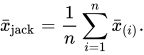
One may ask about the bias and the variance of . From the definition of as the average of the jackknife replicates one could try to calculate explicitly. The bias is a trivial calculation, but the variance of is more involved since the jackknife replicates are not independent.

For the special case of the mean, one can show explicitly that the jackknife estimate equals the usual estimate:
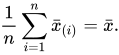
This establishes the identity . Then taking expectations we get , so is unbiased, while taking variance we get . However, these properties do not generally hold for parameters other than the mean.

![{\displaystyle E[{\bar {x}}_{\mathrm {jack} }]=E[{\bar {x}}]=E[x]}](https://wikimedia.org/api/rest_v1/media/math/render/svg/d6b4c0dfb99c56182ce587dca68e4054a22c464d)
![{\displaystyle V[{\bar {x}}_{\mathrm {jack} }]=V[{\bar {x}}]=V[x]/n}](https://wikimedia.org/api/rest_v1/media/math/render/svg/3ccfd3d0e256639b774247153ce1f74fe70e71bb)
This simple example for the case of mean estimation is just to illustrate the construction of a jackknife estimator, while the real subtleties (and the usefulness) emerge for the case of estimating other parameters, such as higher moments than the mean or other functionals of the distribution.
could be used to construct an empirical estimate of the bias of , namely with some suitable factor , although in this case we know that so this construction does not add any meaningful knowledge, but it gives the correct estimation of the bias (which is zero).


A jackknife estimate of the variance of can be calculated from the variance of the jackknife replicates :[3][4]

The left equality defines the estimator and the right equality is an identity that can be verified directly. Then taking expectations we get , so this is an unbiased estimator of the variance of .

![{\displaystyle E[{\widehat {\operatorname {var} }}({\bar {x}})_{\mathrm {jack} }]=V[x]/n=V[{\bar {x}}]}](https://wikimedia.org/api/rest_v1/media/math/render/svg/caceaaa1d30796cf6a296fdb7cf5f3e64f9f57ec)
Estimating the bias of an estimator
[edit]The jackknife technique can be used to estimate (and correct) the bias of an estimator calculated over the entire sample.
Suppose is the target parameter of interest, which is assumed to be some functional of the distribution of . Based on a finite set of observations , which is assumed to consist of i.i.d. copies of , the estimator is constructed:



The value of is sample-dependent, so this value will change from one random sample to another.
By definition, the bias of is as follows:
![{\displaystyle {\text{bias}}({\hat {\theta }})=E[{\hat {\theta }}]-\theta .}](https://wikimedia.org/api/rest_v1/media/math/render/svg/28b2d4fd3492cef9a2e894c9afcb29bf72a2c959)
One may wish to compute several values of from several samples, and average them, to calculate an empirical approximation of , but this is impossible when there are no "other samples" when the entire set of available observations was used to calculate . In this kind of situation the jackknife resampling technique may be of help.
![{\displaystyle E[{\hat {\theta }}]}](https://wikimedia.org/api/rest_v1/media/math/render/svg/4f4d1a469bf57194f821b5e64dd5aa4a8134a3c3)
We construct the jackknife replicates:




where each replicate is a "leave-one-out" estimate based on the jackknife subsample consisting of all but one of the data points:

Then we define their average:
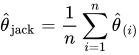
The jackknife estimate of the bias of is given by:

and the resulting bias-corrected jackknife estimate of is given by:

This removes the bias in the special case that the bias is and reduces it to in other cases.[2]


Estimating the variance of an estimator
[edit]The jackknife technique can be also used to estimate the variance of an estimator calculated over the entire sample.
Literature
[edit]- Berger, Y.G. (2007). "A jackknife variance estimator for unistage stratified samples with unequal probabilities". Biometrika. 94 (4): 953–964. doi:10.1093/biomet/asm072.
- Berger, Y.G.; Rao, J.N.K. (2006). "Adjusted jackknife for imputation under unequal probability sampling without replacement". Journal of the Royal Statistical Society, Series B. 68 (3): 531–547. doi:10.1111/j.1467-9868.2006.00555.x.
- Berger, Y.G.; Skinner, C.J. (2005). "A jackknife variance estimator for unequal probability sampling". Journal of the Royal Statistical Society, Series B. 67 (1): 79–89. doi:10.1111/j.1467-9868.2005.00489.x.
- Jiang, J.; Lahiri, P.; Wan, S-M. (2002). "A unified jackknife theory for empirical best prediction with M-estimation". The Annals of Statistics. 30 (6): 1782–810. doi:10.1214/aos/1043351257.
- Jones, H.L. (1974). "Jackknife estimation of functions of stratum means". Biometrika. 61 (2): 343–348. doi:10.2307/2334363. JSTOR 2334363.
- Kish, L.; Frankel, M.R. (1974). "Inference from complex samples". Journal of the Royal Statistical Society, Series B. 36 (1): 1–37.
- Krewski, D.; Rao, J.N.K. (1981). "Inference from stratified samples: properties of the linearization, jackknife and balanced repeated replication methods". The Annals of Statistics. 9 (5): 1010–1019. doi:10.1214/aos/1176345580.
- Quenouille, M.H. (1956). "Notes on bias in estimation". Biometrika. 43 (3–4): 353–360. doi:10.1093/biomet/43.3-4.353.
- Rao, J.N.K.; Shao, J. (1992). "Jackknife variance estimation with survey data under hot deck imputation". Biometrika. 79 (4): 811–822. doi:10.1093/biomet/79.4.811.
- Rao, J.N.K.; Wu, C.F.J.; Yue, K. (1992). "Some recent work on resampling methods for complex surveys". Survey Methodology. 18 (2): 209–217.
- Shao, J. and Tu, D. (1995). The Jackknife and Bootstrap. Springer-Verlag, Inc.
- Tukey, J.W. (1958). "Bias and confidence in not-quite large samples (abstract)". The Annals of Mathematical Statistics. 29 (2): 614.
- Wu, C.F.J. (1986). "Jackknife, Bootstrap and other resampling methods in regression analysis". The Annals of Statistics. 14 (4): 1261–1295. doi:10.1214/aos/1176350142.
Notes
[edit]- ^ Efron 1982, p. 2.
- ^ a b c Cameron & Trivedi 2005, p. 375.
- ^ Efron 1982, p. 14.
- ^ McIntosh, Avery I. "The Jackknife Estimation Method" (PDF). Boston University. Avery I. McIntosh. Archived from the original (PDF) on 2016-05-14. Retrieved 2016-04-30.: p. 3.
References
[edit]- Cameron, Adrian; Trivedi, Pravin K. (2005). Microeconometrics : methods and applications. Cambridge New York: Cambridge University Press. ISBN 9780521848053.
- Efron, Bradley; Stein, Charles (May 1981). "The Jackknife Estimate of Variance". The Annals of Statistics. 9 (3): 586–596. doi:10.1214/aos/1176345462. JSTOR 2240822.
- Efron, Bradley (1982). The jackknife, the bootstrap, and other resampling plans. Philadelphia, PA: Society for Industrial and Applied Mathematics. ISBN 9781611970319.
- Quenouille, Maurice H. (September 1949). "Problems in Plane Sampling". The Annals of Mathematical Statistics. 20 (3): 355–375. doi:10.1214/aoms/1177729989. JSTOR 2236533.
- Quenouille, Maurice H. (1956). "Notes on Bias in Estimation". Biometrika. 43 (3–4): 353–360. doi:10.1093/biomet/43.3-4.353. JSTOR 2332914.
- Tukey, John W. (1958). "Bias and confidence in not quite large samples (abstract)". The Annals of Mathematical Statistics. 29 (2): 614. doi:10.1214/aoms/1177706647.


Jackknife resampling
View on GrokipediaIntroduction and Fundamentals
Definition and Motivation
Jackknife resampling is a non-parametric statistical technique designed to assess the reliability of estimators by generating multiple subsets from an original sample of size , where each subset omits exactly one observation, resulting in such subsets.[2] This approach falls within the broader framework of resampling methods in statistics, which emerged to overcome the shortcomings of traditional parametric techniques that often require strong distributional assumptions about the data.[5] For complex estimators, such as those involving medians or ratios, conventional standard error calculations can fail due to the lack of closed-form expressions or reliance on unverified asymptotic normality, particularly in small or moderate sample sizes.[2] The primary motivation for jackknife resampling lies in its ability to provide empirical approximations of bias and variance without invoking large-sample asymptotic theory, which may not hold reliably for finite datasets.[5] By leveraging the original sample to simulate variability through systematic deletion, it enables statisticians to evaluate estimator performance in scenarios where analytical derivations are infeasible or inaccurate.[2] This method thus bridges the gap between theoretical inference and practical data analysis, offering a robust tool for uncertainty quantification in diverse applications.[5] Key advantages of the jackknife include its computational simplicity relative to more intensive simulation-based alternatives, as it requires only recomputations rather than generating numerous random samples.[2] Additionally, it effectively reduces bias in certain estimators, such as the sample variance, by adjusting for finite-sample effects that traditional formulas overlook.[5] These features make it particularly appealing for scenarios demanding quick, distribution-free assessments of statistical stability.[2]Historical Development
The jackknife resampling technique originated in the mid-20th century as a method for bias reduction in statistical estimation. Maurice Quenouille first introduced a preliminary form of the technique in 1949, applying it to reduce bias in estimators of serial correlation by splitting samples into halves and averaging the results. He further refined and generalized the approach in 1956, extending it to bias correction in ratio estimation and other symmetric estimators through a systematic leave-one-out procedure.[6][7] In 1958, John Tukey built upon Quenouille's work by demonstrating the method's utility for variance estimation and confidence interval construction, while coining the term "jackknife" to evoke the versatility and robustness of a pocket knife as a multi-purpose tool. This naming and expansion marked a key milestone, shifting the jackknife from a niche bias-correction tool to a broader resampling strategy applicable to various estimators.[6] The technique gained further prominence through comprehensive reviews and formalizations in the 1970s. Rupert G. Miller Jr. provided an influential survey in 1974, synthesizing early developments and evaluating the jackknife's effectiveness in bias reduction alongside its emerging role in robust inference. Bradley Efron then formalized and extended the method in his seminal 1979 paper, integrating it with variance estimation and laying groundwork for its incorporation into wider resampling frameworks during the 1980s, as computational advances enabled practical implementations.[6][2]Core Methodology
Basic Procedure
The basic procedure of the delete-one jackknife resampling method involves systematically omitting one observation at a time from the original sample to generate replicates of an estimator. Given an independent and identically distributed sample and an estimator computed from the full sample, the process begins by calculating .[8] For each , the jackknife replicate is then computed by applying the estimator to the reduced sample excluding , that is, .[8] This yields a set of jackknife replicates . The jackknife sample mean is defined as . Pseudo-values provide a transformed set of values derived from the replicates, facilitating further statistical analysis by treating them analogously to independent observations. Introduced by Tukey, the pseudo-value for the -th observation is given byfunction jackknife_replicates([data](/page/Data), [estimator](/page/Estimator)):
n = length([data](/page/Data))
theta_hat = [estimator](/page/Estimator)([data](/page/Data)) # Full sample estimate
replicates = [array](/page/Array) of [size](/page/Size) n
for i in 1 to n:
reduced_data = [data](/page/Data) without [data](/page/Data)[i]
replicates[i] = [estimator](/page/Estimator)(reduced_data)
return theta_hat, replicates
# Optional: Compute pseudo-values
function pseudo_values(theta_hat, replicates, n):
pv = [array](/page/Array) of [size](/page/Size) n
for i in 1 to n:
pv[i] = n * theta_hat - (n - 1) * replicates[i]
return pv
Pseudo-Values and Jackknife Estimates
In jackknife resampling, pseudo-values are derived from the full-sample estimator and the leave-one-out estimators , where is computed by omitting the -th observation from the sample of size . The -th pseudo-value is given byEstimation Techniques
Bias Correction
In jackknife resampling, bias correction is achieved by estimating the bias of an estimator and subtracting it to obtain a corrected version, with pseudo-values serving as the computational basis for deriving these estimates.[11] The jackknife estimate of bias, denoted , is given by , where is the sample size, is the estimator computed from the full sample, and is the average of the leave-one-out estimators , each omitting the -th observation. To derive this, consider the influence of a single observation on the estimator. For a leave-one-out sample of size , the expected value of approximates the bias expansion for smaller samples. Specifically, if the bias of based on observations is , then averaging over the leave-one-out estimates yields . Substituting into the formula gives , isolating and scaling the leading term, removing the first-order bias contribution. The bias-corrected jackknife estimator is then , which simplifies to .[11] Theoretically, this correction is justified through the asymptotic expansion of the bias, assuming the estimator is consistent and the data are independent with finite moments. Under these conditions, the jackknife reduces the bias from to . It is particularly effective for mildly biased estimators, such as the sample variance computed as , where the first-order bias is removed, though it does not address higher-order biases.Variance Estimation
The jackknife method provides an estimate of the variance of a point estimator derived from a sample of size by computing leave-one-out replicates for , where each is the estimator based on the sample excluding the -th observation. The jackknife variance estimator is then given byPractical Examples
Univariate Mean Estimation
Jackknife resampling provides a practical illustration in the context of estimating the population mean from a univariate sample drawn independently from an unknown distribution , where the estimator is the sample mean .[12] The jackknife procedure generates replicates by omitting one observation at a time, yielding for .[12] Consider a small dataset with and values . The original sample mean is . The jackknife replicates are computed as follows: omitting gives ; omitting gives ; omitting gives . The average of these replicates is .[14] Applying the general jackknife formulas to this case, the bias estimate is .[12] The variance estimate is .[12] These results are summarized in the table below:| 1 | 1 | 2.5 | 0.5 |
| 2 | 2 | 2 | 0 |
| 3 | 3 | 1.5 | -0.5 |
Linear Regression Coefficients
In linear regression, the model is specified as $ \mathbf{Y} = \mathbf{X} \boldsymbol{\beta} + \boldsymbol{\varepsilon} $, where $ \mathbf{Y} $ is an $ n \times 1 $ response vector, $ \mathbf{X} $ is an $ n \times p $ design matrix of predictors, $ \boldsymbol{\beta} $ is a $ p \times 1 $ vector of unknown coefficients, and $ \boldsymbol{\varepsilon} $ is an error vector with mean zero. The ordinary least-squares estimator is $ \hat{\boldsymbol{\beta}} = (\mathbf{X}^T \mathbf{X})^{-1} \mathbf{X}^T \mathbf{Y} $.[15] The jackknife procedure for coefficients involves refitting the model $ n $ times, each time omitting one observation to obtain $ \hat{\boldsymbol{\beta}}{-i} $ for $ i = 1, \dots, n $. Focusing on a single coefficient for simplicity, such as the slope $ \hat{\beta}j $, the leave-one-out estimates $ \hat{\beta}{j,-i} $ are used to compute pseudo-values $ \beta{j,i}^* = n \hat{\beta}j - (n-1) \hat{\beta}{j,-i} $. The jackknife estimate of $ \beta_j $ is the average of these pseudo-values, which corrects for bias as $ \hat{\beta}j^{JK} = n \bar{\hat{\beta}}{j,(-.)} - (n-1) \hat{\beta}j $, where $ \bar{\hat{\beta}}{j,(-.)} = \frac{1}{n} \sum_{i=1}^n \hat{\beta}{j,-i} $. The estimated bias is $ n (\bar{\hat{\beta}}{j,(-.)} - \hat{\beta}j ) $, and the variance is $ \widehat{\mathrm{Var}}(\hat{\beta}j) = \frac{n-1}{n} \sum{i=1}^n (\hat{\beta}{j,-i} - \bar{\hat{\beta}}_{j,(-.)})^2 $. This delete-one approach extends the univariate case by requiring full model refits at each step.[15] For illustration, consider a simulated dataset with $ n=10 $ observations and $ p=2 $ predictors, where the full-sample slope for the first predictor is $ \hat{\beta}1 = 2.0 $. The leave-one-out slope estimates $ \hat{\beta}{1,-i} $ are shown in the table below, along with deviations from the average $ \bar{\hat{\beta}}_{1,(-.)} = 2.0 $.| $ i $ | $ \hat{\beta}_{1,-i} $ | Deviation |
|---|---|---|
| 1 | 1.95 | -0.05 |
| 2 | 2.05 | 0.05 |
| 3 | 1.90 | -0.10 |
| 4 | 2.10 | 0.10 |
| 5 | 2.00 | 0.00 |
| 6 | 1.85 | -0.15 |
| 7 | 2.15 | 0.15 |
| 8 | 2.00 | 0.00 |
| 9 | 1.95 | -0.05 |
| 10 | 2.05 | 0.05 |