



Community hub
Polar amplification
View on Wikipedia
Polar amplification is the phenomenon that any change in the net radiation balance (for example greenhouse intensification) tends to produce a larger change in temperature near the poles than in the planetary average.[1] This is commonly referred to as the ratio of polar warming to tropical warming. On a planet with an atmosphere that can restrict emission of longwave radiation to space (a greenhouse effect), surface temperatures will be warmer than a simple planetary equilibrium temperature calculation would predict. Where the atmosphere or an extensive ocean is able to transport heat polewards, the poles will be warmer and equatorial regions cooler than their local net radiation balances would predict.[2] The poles will experience the most cooling when the global-mean temperature is lower relative to a reference climate; alternatively, the poles will experience the greatest warming when the global-mean temperature is higher.[1]
In the extreme, the planet Venus is thought to have experienced a very large increase in greenhouse effect over its lifetime,[3] so much so that its poles have warmed sufficiently to render its surface temperature effectively isothermal (no difference between poles and equator).[4][5] On Earth, water vapor and trace gasses provide a lesser greenhouse effect, and the atmosphere and extensive oceans provide efficient poleward heat transport. Both palaeoclimate changes and recent global warming changes have exhibited strong polar amplification, as described below.
Arctic amplification is polar amplification of the Earth's North Pole only; Antarctic amplification is that of the South Pole.
History
[edit]An observation-based study related to Arctic amplification was published in 1969 by Mikhail Budyko,[6] and the study conclusion has been summarized as "Sea ice loss affects Arctic temperatures through the surface albedo feedback."[7][8] The same year, a similar model was published by William D. Sellers.[9] Both studies attracted significant attention since they hinted at the possibility for a runaway positive feedback within the global climate system.[10] In 1975, Manabe and Wetherald published the first somewhat plausible general circulation model that looked at the effects of an increase of greenhouse gas. Although confined to less than one-third of the globe, with a "swamp" ocean and only land surface at high latitudes, it showed an Arctic warming faster than the tropics (as have all subsequent models).[11]
Amplification
[edit]Amplifying mechanisms
[edit]Feedbacks associated with sea ice and snow cover are widely cited as one of the principal causes of terrestrial polar amplification.[12][13][14] These feedbacks are particularly noted in local polar amplification,[15] although recent work has shown that the lapse rate feedback is likely equally important to the ice-albedo feedback for Arctic amplification.[16] Supporting this idea, large-scale amplification is also observed in model worlds with no ice or snow.[17] It appears to arise both from a (possibly transient) intensification of poleward heat transport and more directly from changes in the local net radiation balance.[17] Local radiation balance is crucial because an overall decrease in outgoing longwave radiation will produce a larger relative increase in net radiation near the poles than near the equator.[16] Thus, between the lapse rate feedback and changes in the local radiation balance, much of polar amplification can be attributed to changes in outgoing longwave radiation.[15][18] This is especially true for the Arctic, whereas the elevated terrain in Antarctica limits the influence of the lapse rate feedback.[16][19]
Some examples of climate system feedbacks thought to contribute to recent polar amplification include the reduction of snow cover and sea ice, changes in atmospheric and ocean circulation, the presence of anthropogenic soot in the Arctic environment, and increases in cloud cover and water vapor.[13] CO2 forcing has also been attributed to polar amplification.[20] Most studies connect sea ice changes to polar amplification.[13] Both ice extent and thickness impact polar amplification. Climate models with smaller baseline sea ice extent and thinner sea ice coverage exhibit stronger polar amplification.[21] Some models of modern climate exhibit Arctic amplification without changes in snow and ice cover.[22]
The individual processes contributing to polar warming are critical to understanding climate sensitivity.[23] Polar warming also affects many ecosystems, including marine and terrestrial ecosystems, climate systems, and human populations.[20] Polar amplification is largely driven by local polar processes with hardly any remote forcing, whereas polar warming is regulated by tropical and midlatitude forcing.[20] These impacts of polar amplification have led to continuous research in the face of global warming.
Ocean circulation
[edit]It has been estimated that 70% of global wind energy is transferred to the ocean and takes place within the Antarctic Circumpolar Current (ACC).[24] Eventually, upwelling due to wind-stress transports cold Antarctic waters through the Atlantic surface current, while warming them over the equator, and into the Arctic environment. This is especially noticed in high latitudes.[21] Thus, warming in the Arctic depends on the efficiency of the global ocean transport and plays a role in the polar see-saw effect.[24]
Decreased oxygen and low-pH during La Niña are processes that correlate with decreased primary production and a more pronounced poleward flow of ocean currents.[25] It has been proposed that the mechanism of increased Arctic surface air temperature anomalies during La Niña periods of ENSO may be attributed to the Tropically Excited Arctic Warming Mechanism (TEAM), when Rossby waves propagate more poleward, leading to wave dynamics and an increase in downward infrared radiation.[1][26]
Amplification factor
[edit]Polar amplification is quantified in terms of a polar amplification factor, generally defined as the ratio of some change in a polar temperature to a corresponding change in a broader average temperature:
- ,
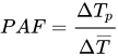
where is a change in polar temperature and is, for example, a corresponding change in a global mean temperature.


Common implementations[27][28] define the temperature changes directly as the anomalies in surface air temperature relative to a recent reference interval (typically 30 years). Others have used the ratio of the variances of surface air temperature over an extended interval.[29]
Amplification phase
[edit]
It is observed that Arctic and Antarctic warming commonly proceed out of phase because of orbital forcing, resulting in the so-called polar see-saw effect.[30]
Paleoclimate polar amplification
[edit]The glacial / interglacial cycles of the Pleistocene provide extensive palaeoclimate evidence of polar amplification, both from the Arctic and the Antarctic.[28] In particular, the temperature rise since the last glacial maximum 20,000 years ago provides a clear picture. Proxy temperature records from the Arctic (Greenland) and from the Antarctic indicate polar amplification factors on the order of 2.0.[28]
Recent Arctic amplification
[edit].jpg)
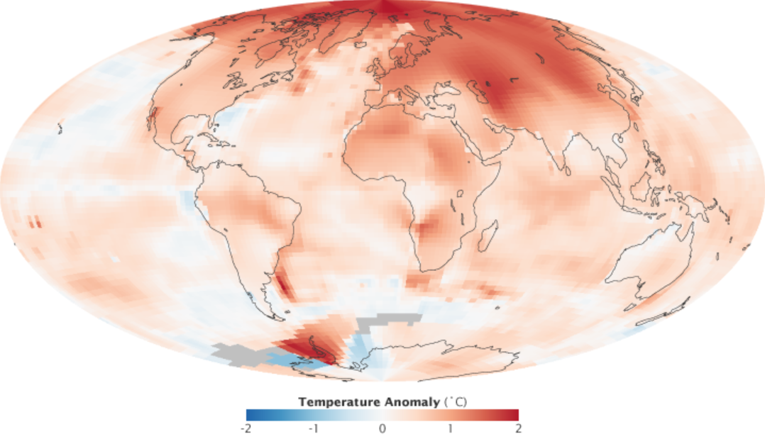
Suggested mechanisms leading to the observed Arctic amplification include Arctic sea ice decline (open water reflects less sunlight than sea ice), atmospheric heat transport from the equator to the Arctic,[32] and the lapse rate feedback.[16]
The Arctic was historically described as warming twice as fast as the global average,[33] but this estimate was based on older observations which missed the more recent acceleration. By 2021, enough data was available to show that the Arctic had warmed three times as fast as the globe - 3.1°C between 1971 and 2019, as opposed to the global warming of 1°C over the same period.[34] Moreover, this estimate defines the Arctic as everything above 60th parallel north, or a full third of the Northern Hemisphere: in 2021–2022, it was found that since 1979, the warming within the Arctic Circle itself (above the 66th parallel) has been nearly four times faster than the global average.[35][36] Within the Arctic Circle itself, even greater Arctic amplification occurs in the Barents Sea area, with hotspots around West Spitsbergen Current: weather stations located on its path record decadal warming up to seven times faster than the global average.[37][38] This has fuelled concerns that unlike the rest of the Arctic sea ice, ice cover in the Barents Sea may permanently disappear even around 1.5 degrees of global warming.[39][40]
The acceleration of Arctic amplification has not been linear: a 2022 analysis found that it occurred in two sharp steps, with the former around 1986, and the latter after 2000.[41] The first acceleration is attributed to the increase in anthropogenic radiative forcing in the region, which is in turn likely connected to the reductions in stratospheric sulfur aerosols pollution in Europe in the 1980s in order to combat acid rain. Since sulphate aerosols have a cooling effect, their absence is likely to have increased Arctic temperatures by up to 0.5 degrees Celsius.[42][43] The second acceleration has no known cause,[34] which is why it did not show up in any climate models. It is likely to be an example of multi-decadal natural variability, like the suggested link between Arctic temperatures and Atlantic Multi-decadal Oscillation (AMO),[44] in which case it can be expected to reverse in the future. However, even the first increase in Arctic amplification was only accurately simulated by a fraction of the current CMIP6 models.[41] Recent studies show the Arctic has warmed nearly four times faster than the global average since 1979, with areas like the Barents Sea experiencing rates up to seven times higher, highlighting the urgent need to address polar climate change.[45]
Possible impacts on mid-latitude weather
[edit]Since the early 2000s, climate models have consistently identified that global warming will gradually push jet streams poleward. In 2008, this was confirmed by observational evidence, which proved that from 1979 to 2001, the northern jet stream moved northward at an average rate of 2.01 kilometres (1.25 mi) per year, with a similar trend in the southern hemisphere jet stream.[46][47] Climate scientists have hypothesized that the jet stream will also gradually weaken as a result of global warming. Trends such as Arctic sea ice decline, reduced snow cover, evapotranspiration patterns, and other weather anomalies have caused the Arctic to heat up faster than other parts of the globe, in what is known as the Arctic amplification. In 2021–2022, it was found that since 1979, the warming within the Arctic Circle has been nearly four times faster than the global average,[48][49] and some hotspots in the Barents Sea area warmed up to seven times faster than the global average.[50][51] While the Arctic remains one of the coldest places on Earth today, the temperature gradient between it and the warmer parts of the globe will continue to diminish with every decade of global warming as the result of this amplification. If this gradient has a strong influence on the jet stream, then it will eventually become weaker and more variable in its course, which would allow more cold air from the polar vortex to leak mid-latitudes and slow the progression of Rossby waves, leading to more persistent and more extreme weather.[52]
The hypothesis above is closely associated with Jennifer Francis, who had first proposed it in a 2012 paper co-authored by Stephen J. Vavrus.[52] While some paleoclimate reconstructions have suggested that the polar vortex becomes more variable and causes more unstable weather during periods of warming back in 1997,[53] this was contradicted by climate modelling, with PMIP2 simulations finding in 2010 that the Arctic Oscillation (AO) was much weaker and more negative during the Last Glacial Maximum, and suggesting that warmer periods have stronger positive phase AO, and thus less frequent leaks of the polar vortex air.[54] However, a 2012 review in the Journal of the Atmospheric Sciences noted that "there [has been] a significant change in the vortex mean state over the twenty-first century, resulting in a weaker, more disturbed vortex.",[55] which contradicted the modelling results but fit the Francis-Vavrus hypothesis. Additionally, a 2013 study noted that the then-current CMIP5 tended to strongly underestimate winter blocking trends,[56] and other 2012 research had suggested a connection between declining Arctic sea ice and heavy snowfall during midlatitude winters.[57]
In 2013, further research from Francis connected reductions in the Arctic sea ice to extreme summer weather in the northern mid-latitudes,[58] while other research from that year identified potential linkages between Arctic sea ice trends and more extreme rainfall in the European summer.[59] At the time, it was also suggested that this connection between Arctic amplification and jet stream patterns was involved in the formation of Hurricane Sandy[60] and played a role in the early 2014 North American cold wave.[61][62] In 2015, Francis' next study concluded that highly amplified jet-stream patterns are occurring more frequently in the past two decades. Hence, continued heat-trapping emissions favour increased formation of extreme events caused by prolonged weather conditions.[63]
Studies published in 2017 and 2018 identified stalling patterns of Rossby waves in the northern hemisphere jet stream as the culprit behind other almost stationary extreme weather events, such as the 2018 European heatwave, the 2003 European heat wave, 2010 Russian heat wave or the 2010 Pakistan floods, and suggested that these patterns were all connected to Arctic amplification.[64][65] Further work from Francis and Vavrus that year suggested that amplified Arctic warming is observed as stronger in lower atmospheric areas because the expanding process of warmer air increases pressure levels which decreases poleward geopotential height gradients. As these gradients are the reason that cause west to east winds through the thermal wind relationship, declining speeds are usually found south of the areas with geopotential increases.[66] In 2017, Francis explained her findings to the Scientific American: "A lot more water vapor is being transported northward by big swings in the jet stream. That's important because water vapor is a greenhouse gas just like carbon dioxide and methane. It traps heat in the atmosphere. That vapor also condenses as droplets we know as clouds, which themselves trap more heat. The vapor is a big part of the amplification story—a big reason the Arctic is warming faster than anywhere else."[67]
In a 2017 study conducted by climatologist Judah Cohen and several of his research associates, Cohen wrote that "[the] shift in polar vortex states can account for most of the recent winter cooling trends over Eurasian midlatitudes".[68] A 2018 paper from Vavrus and others linked Arctic amplification to more persistent hot-dry extremes during the midlatitude summers, as well as the midlatitude winter continental cooling.[69] Another 2017 paper estimated that when the Arctic experiences anomalous warming, primary production in North America goes down by between 1% and 4% on average, with some states suffering up to 20% losses.[70] A 2021 study found that a stratospheric polar vortex disruption is linked with extreme cold winter weather across parts of Asia and North America, including the February 2021 North American cold wave.[71][72] Another 2021 study identified a connection between the Arctic sea ice loss and the increased size of wildfires in the Western United States.[73]
However, because the specific observations are considered short-term observations, there is considerable uncertainty in the conclusions. Climatology observations require several decades to definitively distinguish various forms of natural variability from climate trends.[74] This point was stressed by reviews in 2013[75] and in 2017.[76] A study in 2014 concluded that Arctic amplification significantly decreased cold-season temperature variability over the northern hemisphere in recent decades. Cold Arctic air intrudes into the warmer lower latitudes more rapidly today during autumn and winter, a trend projected to continue in the future except during summer, thus calling into question whether winters will bring more cold extremes.[77] A 2019 analysis of a data set collected from 35 182 weather stations worldwide, including 9116 whose records go beyond 50 years, found a sharp decrease in northern midlatitude cold waves since the 1980s.[78]
Moreover, a range of long-term observational data collected during the 2010s and published in 2020 suggests that the intensification of Arctic amplification since the early 2010s was not linked to significant changes on mid-latitude atmospheric patterns.[79][80] State-of-the-art modelling research of PAMIP (Polar Amplification Model Intercomparison Project) improved upon the 2010 findings of PMIP2; it found that sea ice decline would weaken the jet stream and increase the probability of atmospheric blocking, but the connection was very minor, and typically insignificant next to interannual variability.[81][82] In 2022, a follow-up study found that while the PAMIP average had likely underestimated the weakening caused by sea ice decline by 1.2 to 3 times, even the corrected connection still amounts to only 10% of the jet stream's natural variability.[83]
Additionally, a 2021 study found that while jet streams had indeed slowly moved polewards since 1960 as was predicted by models, they did not weaken, in spite of a small increase in waviness.[84] A 2022 re-analysis of the aircraft observational data collected over 2002–2020 suggested that the North Atlantic jet stream had actually strengthened.[85] Finally, a 2021 study was able to reconstruct jet stream patterns over the past 1,250 years based on Greenland ice cores, and found that all of the recently observed changes remain within range of natural variability: the earliest likely time of divergence is in 2060, under the Representative Concentration Pathway 8.5 which implies continually accelerating greenhouse gas emissions.[86]See also
[edit]References
[edit]- ^ a b c Lee, Sukyoung (January 2014). "A theory for polar amplification from a general circulation perspective" (PDF). Asia-Pacific Journal of the Atmospheric Sciences. 50 (1): 31–43. Bibcode:2014APJAS..50...31L. doi:10.1007/s13143-014-0024-7. S2CID 20639425. Archived from the original (PDF) on 2016-03-04. Retrieved 2014-05-01.
- ^ Pierrehumbert, R. T. (2010). Principles of Planetary Climate. Cambridge University Press. ISBN 978-0-521-86556-2.
- ^ Kasting, J. F. (1988). "Runaway and moist greenhouse atmospheres and the evolution of Earth and Venus". Icarus. 74 (3): 472–94. Bibcode:1988Icar...74..472K. doi:10.1016/0019-1035(88)90116-9. PMID 11538226.
- ^ Williams, David R. (15 April 2005). "Venus Fact Sheet". NASA. Retrieved 2007-10-12.
- ^ Lorenz, Ralph D.; Lunine, Jonathan I.; Withers, Paul G.; McKay, Christopher P. (2001). "Titan, Mars and Earth: Entropy Production by Latitudinal Heat Transport" (PDF). Ames Research Center, University of Arizona Lunar and Planetary Laboratory. Retrieved 2007-08-21.
- ^ Budyko, M.I. (1969). "The effect of solar radiation variations on the climate of the Earth". Tellus. 21 (5): 611–9. Bibcode:1969Tell...21..611B. doi:10.3402/tellusa.v21i5.10109. S2CID 21745322.
- ^ Cvijanovic, Ivana; Caldeira, Ken (2015). "Atmospheric impacts of sea ice decline in CO2 induced global warming" (PDF). Climate Dynamics. 44 (5–6): 1173–86. Bibcode:2015ClDy...44.1173C. doi:10.1007/s00382-015-2489-1. S2CID 106405448.
- ^ "Ice in Action: Sea ice at the North Pole has something to say about climate change". YaleScientific. 2016.
- ^ Sellers, William D. (1969). "A Global Climatic Model Based on the Energy Balance of the Earth-Atmosphere System". Journal of Applied Meteorology. 8 (3): 392–400. Bibcode:1969JApMe...8..392S. doi:10.1175/1520-0450(1969)008<0392:AGCMBO>2.0.CO;2.
- ^ Oldfield, Jonathan D. (2016). "Mikhail Budyko's (1920–2001) contributions to Global Climate Science: from heat balances to climate change and global ecology". Advanced Review. 7 (5): 682–692. Bibcode:2016WIRCC...7..682O. doi:10.1002/wcc.412.
- ^ Manabe, Syukoro; Wetherald, Richard T. (1975). "The Effects of Doubling the CO2 Concentration on the Climate of a General Circulation Model". Journal of the Atmospheric Sciences. 32 (1): 3–15. Bibcode:1975JAtS...32....3M. doi:10.1175/1520-0469(1975)032<0003:TEODTC>2.0.CO;2.
- ^ Hansen J, Sato M, Ruedy R (1997). "Radiative forcing and climate response". Journal of Geophysical Research: Atmospheres. 102 (D6): 6831–64. Bibcode:1997JGR...102.6831H. doi:10.1029/96jd03436.
- ^ a b c "IPCC AR5 – Near-term Climate Change: Projections and Predictability (Chapter 11 / page 983 )" (PDF). 2013.
- ^ Pistone, Kristina; Eisenman, Ian; Ramanathan, Veerabhadran (2019). "Radiative Heating of an Ice-Free Arctic Ocean". Geophysical Research Letters. 46 (13): 7474–7480. Bibcode:2019GeoRL..46.7474P. doi:10.1029/2019GL082914. S2CID 197572148.
- ^ a b Bekryaev, Roman V.; Polyakov, Igor V.; Alexeev, Vladimir A. (2010-07-15). "Role of Polar Amplification in Long-Term Surface Air Temperature Variations and Modern Arctic Warming". Journal of Climate. 23 (14): 3888–3906. Bibcode:2010JCli...23.3888B. doi:10.1175/2010JCLI3297.1. ISSN 0894-8755.
- ^ a b c d Goosse, Hugues; Kay, Jennifer E.; Armour, Kyle C.; Bodas-Salcedo, Alejandro; Chepfer, Helene; Docquier, David; Jonko, Alexandra; Kushner, Paul J.; Lecomte, Olivier; Massonnet, François; Park, Hyo-Seok; Pithan, Felix; Svensson, Gunilla; Vancoppenolle, Martin (December 2018). "Quantifying climate feedbacks in polar regions". Nature Communications. 9 (1): 1919. Bibcode:2018NatCo...9.1919G. doi:10.1038/s41467-018-04173-0. PMC 5953926. PMID 29765038.
- ^ a b Alexeev VA, Langen PL, Bates JR (2005). "Polar amplification of surface warming on an aquaplanet in "ghost forcing" experiments without sea ice feedbacks". Climate Dynamics. 24 (7–8): 655–666. Bibcode:2005ClDy...24..655A. doi:10.1007/s00382-005-0018-3. S2CID 129600712.
- ^ Payne, Ashley E.; Jansen, Malte F.; Cronin, Timothy W. (2015). "Conceptual model analysis of the influence of temperature feedbacks on polar amplification". Geophysical Research Letters. 42 (21): 9561–9570. Bibcode:2015GeoRL..42.9561P. doi:10.1002/2015GL065889. ISSN 1944-8007.
- ^ Hahn, L. C.; Armour, K. C.; Battisti, D. S.; Donohoe, A.; Pauling, A. G.; Bitz, C. M. (28 August 2020). "Antarctic Elevation Drives Hemispheric Asymmetry in Polar Lapse Rate Climatology and Feedback". Geophysical Research Letters. 47 (16). Bibcode:2020GeoRL..4788965H. doi:10.1029/2020GL088965. S2CID 222009674.
- ^ a b c Stuecker, Malte F.; Bitz, Cecilia M.; Armour, Kyle C.; Proistosescu, Cristian; Kang, Sarah M.; Xie, Shang Ping; Kim, Doyeon; McGregor, Shayne; Zhang, Wenjun; Zhao, Sen; Cai, Wenju (December 2018). "Polar amplification dominated by local forcing and feedbacks". Nature Climate Change. 8 (12): 1076–1081. Bibcode:2018NatCC...8.1076S. doi:10.1038/s41558-018-0339-y. ISSN 1758-6798. S2CID 92195853.
- ^ a b Holland, M. M.; Bitz, C. M. (2003-09-01). "Polar amplification of climate change in coupled models". Climate Dynamics. 21 (3): 221–232. Bibcode:2003ClDy...21..221H. doi:10.1007/s00382-003-0332-6. ISSN 1432-0894. S2CID 17003665.
- ^ Pithan, Felix; Mauritsen, Thorsten (February 2, 2014). "Arctic amplification dominated by temperature feedbacks in contemporary climate models". Nature Geoscience. 7 (3): 181–4. Bibcode:2014NatGe...7..181P. doi:10.1038/ngeo2071. S2CID 140616811.
- ^ Taylor, Patrick C.; Cai, Ming; Hu, Aixue; Meehl, Jerry; Washington, Warren; Zhang, Guang J. (2013-09-09). "A Decomposition of Feedback Contributions to Polar Warming Amplification". Journal of Climate. 26 (18). American Meteorological Society: 7023–7043. Bibcode:2013JCli...26.7023T. doi:10.1175/jcli-d-12-00696.1. ISSN 0894-8755.
- ^ a b Petr Chylek; Chris K. Folland; Glen Lesins; Manvendra K. Dubey (February 3, 2010). "Twentieth century bipolar seesaw of the Arctic and Antarctic surface air temperatures" (PDF). Geophysical Research Letters. 12 (8): 4015–22. Bibcode:2010GeoRL..37.8703C. doi:10.1029/2010GL042793. S2CID 18491097. Archived from the original (PDF) on February 20, 2014. Retrieved May 1, 2014.
- ^ Sung Hyun Nam; Hey-Jin Kim; Uwe Send (November 23, 2011). "Amplification of hypoxic and acidic events by La Niña conditions on the continental shelf off California". Geophysical Research Letters. 83 (22): L22602. Bibcode:2011GeoRL..3822602N. doi:10.1029/2011GL049549. S2CID 55150106.
- ^ Sukyoung Lee (June 2012). "Testing of the Tropically Excited Arctic Warming Mechanism (TEAM) with Traditional El Niño and La Niña". Journal of Climate. 25 (12): 4015–22. Bibcode:2012JCli...25.4015L. doi:10.1175/JCLI-D-12-00055.1. S2CID 91176052.
- ^ Masson-Delmotte, V.; M. Kageyama; P. Braconnot; S. Charbit; G. Krinner; C. Ritz; E. Guilyardi; et al. (2006). "Past and future polar amplification of climate change: climate model intercomparisons and ice-core constraints". Climate Dynamics. 26 (5): 513–529. Bibcode:2006ClDy...26..513M. doi:10.1007/s00382-005-0081-9. S2CID 2370836.
- ^ a b c James Hansen; Makiko Sato; Gary Russell; Pushker Kharecha (September 2013). "Climate sensitivity, sea level and atmospheric carbon dioxide". Philosophical Transactions of the Royal Society A. 371 (2001). arXiv:1211.4846. Bibcode:2013RSPTA.37120294H. doi:10.1098/rsta.2012.0294. PMC 3785813. PMID 24043864.
- ^ Kobashi, T.; Shindell, D. T.; Kodera, K.; Box, J. E.; Nakaegawa, T.; Kawamura, K. (2013). "On the origin of multidecadal to centennial Greenland temperature anomalies over the past 800 yr". Climate of the Past. 9 (2): 583–596. Bibcode:2013CliPa...9..583K. doi:10.5194/cp-9-583-2013. hdl:2060/20150002680.
- ^ Kyoung-nam Jo; Kyung Sik Woo; Sangheon Yi; Dong Yoon Yang; Hyoun Soo Lim; Yongjin Wang; Hai Cheng; R. Lawrence Edwards (March 30, 2014). "Mid-latitude interhemispheric hydrologic seesaw over the past 550,000 years". Nature. 508 (7496): 378–382. Bibcode:2014Natur.508..378J. doi:10.1038/nature13076. PMID 24695222. S2CID 2096406.
- ^ "Thermodynamics: Albedo". NSIDC.
- ^ "Arctic amplification". NASA. 2013.
- ^ "Polar Vortex: How the Jet Stream and Climate Change Bring on Cold Snaps". InsideClimate News. 2018-02-02. Retrieved 2018-11-24.
- ^ a b "Arctic warming three times faster than the planet, report warns". Phys.org. 2021-05-20. Retrieved 6 October 2022.
- ^ Rantanen, Mika; Karpechko, Alexey Yu; Lipponen, Antti; Nordling, Kalle; Hyvärinen, Otto; Ruosteenoja, Kimmo; Vihma, Timo; Laaksonen, Ari (11 August 2022). "The Arctic has warmed nearly four times faster than the globe since 1979". Communications Earth & Environment. 3 (1): 168. Bibcode:2022ComEE...3..168R. doi:10.1038/s43247-022-00498-3. hdl:11250/3115996. ISSN 2662-4435. S2CID 251498876.
- ^ "The Arctic is warming four times faster than the rest of the world". 2021-12-14. Retrieved 6 October 2022.
- ^ Isaksen, Ketil; Nordli, Øyvind; et al. (15 June 2022). "Exceptional warming over the Barents area". Scientific Reports. 12 (1): 9371. Bibcode:2022NatSR..12.9371I. doi:10.1038/s41598-022-13568-5. PMC 9200822. PMID 35705593. S2CID 249710630.
- ^ Damian Carrington (2022-06-15). "New data reveals extraordinary global heating in the Arctic". The Guardian. Retrieved 7 October 2022.
- ^ Armstrong McKay, David; Abrams, Jesse; Winkelmann, Ricarda; Sakschewski, Boris; Loriani, Sina; Fetzer, Ingo; Cornell, Sarah; Rockström, Johan; Staal, Arie; Lenton, Timothy (9 September 2022). "Exceeding 1.5°C global warming could trigger multiple climate tipping points". Science. 377 (6611) eabn7950. doi:10.1126/science.abn7950. hdl:10871/131584. ISSN 0036-8075. PMID 36074831. S2CID 252161375.
- ^ Armstrong McKay, David (9 September 2022). "Exceeding 1.5°C global warming could trigger multiple climate tipping points – paper explainer". climatetippingpoints.info. Retrieved 2 October 2022.
- ^ a b Chylek, Petr; Folland, Chris; Klett, James D.; Wang, Muyin; Hengartner, Nick; Lesins, Glen; Dubey, Manvendra K. (25 June 2022). "Annual Mean Arctic Amplification 1970–2020: Observed and Simulated by CMIP6 Climate Models". Geophysical Research Letters. 49 (13). Bibcode:2022GeoRL..4999371C. doi:10.1029/2022GL099371. S2CID 250097858.
- ^ Acosta Navarro, J.C.; Varma, V.; Riipinen, I.; Seland, Ø.; Kirkevåg, A.; Struthers, H.; Iversen, T.; Hansson, H.-C.; Ekman, A. M. L. (14 March 2016). "Amplification of Arctic warming by past air pollution reductions in Europe". Nature Geoscience. 9 (4): 277–281. Bibcode:2016NatGe...9..277A. doi:10.1038/ngeo2673.
- ^ Harvey, C. (14 March 2016). "How cleaner air could actually make global warming worse". Washington Post.
- ^ Chylek, Petr; Folland, Chris K.; Lesins, Glen; Dubey, Manvendra K.; Wang, Muyin (16 July 2009). "Arctic air temperature change amplification and the Atlantic Multidecadal Oscillation". Geophysical Research Letters. 36 (14): L14801. Bibcode:2009GeoRL..3614801C. CiteSeerX 10.1.1.178.6926. doi:10.1029/2009GL038777. S2CID 14013240.
- ^ Rantanen, Mika; Karpechko, Alexey Yu.; Lipponen, Antti; Nordling, Kalle; Hyvärinen, Otto; Ruosteenoja, Kimmo; Vihma, Timo; Laaksonen, Ari (2022-08-11). "The Arctic has warmed nearly four times faster than the globe since 1979". Communications Earth & Environment. 3 (1). doi:10.1038/s43247-022-00498-3. hdl:11250/3115996. ISSN 2662-4435.
- ^ Archer, Cristina L.; Caldeira, Ken (18 April 2008). "Historical trends in the jet streams". Geophysical Research Letters. 35 (8). Bibcode:2008GeoRL..35.8803A. doi:10.1029/2008GL033614. S2CID 59377392.
- ^ "Jet stream found to be permanently drifting north". Associated Press. 2008-04-18. Archived from the original on 17 August 2016. Retrieved 7 October 2022.
- ^ Rantanen, Mika; Karpechko, Alexey Yu; Lipponen, Antti; Nordling, Kalle; Hyvärinen, Otto; Ruosteenoja, Kimmo; Vihma, Timo; Laaksonen, Ari (11 August 2022). "The Arctic has warmed nearly four times faster than the globe since 1979". Communications Earth & Environment. 3 (1): 168. Bibcode:2022ComEE...3..168R. doi:10.1038/s43247-022-00498-3. hdl:11250/3115996. ISSN 2662-4435. S2CID 251498876.
- ^ "The Arctic is warming four times faster than the rest of the world". Science Magazine. 2021-12-14. Archived from the original on 8 November 2023. Retrieved 6 October 2022.
- ^ Isaksen, Ketil; Nordli, Øyvind; et al. (15 June 2022). "Exceptional warming over the Barents area". Scientific Reports. 12 (1): 9371. Bibcode:2022NatSR..12.9371I. doi:10.1038/s41598-022-13568-5. PMC 9200822. PMID 35705593.
- ^ Damian Carrington (2022-06-15). "New data reveals extraordinary global heating in the Arctic". The Guardian. Archived from the original on 1 October 2023. Retrieved 7 October 2022.
- ^ a b Francis, Jennifer A.; Vavrus, Stephen J. (2012). "Evidence linking Arctic amplification to extreme weather in mid-latitudes". Geophysical Research Letters. 39 (6): L06801. Bibcode:2012GeoRL..39.6801F. CiteSeerX 10.1.1.419.8599. doi:10.1029/2012GL051000. S2CID 15383119.
- ^ Zielinski, G.; Mershon, G. (1997). "Paleoenvironmental implications of the insoluble microparticle record in the GISP2 (Greenland) ice core during the rapidly changing climate of the Pleistocene-Holocene transition". Bulletin of the Geological Society of America. 109 (5): 547–559. Bibcode:1997GSAB..109..547Z. doi:10.1130/0016-7606(1997)109<0547:piotim>2.3.co;2.
- ^ Lue, J.-M.; Kim, S.-J.; Abe-Ouchi, A.; Yu, Y.; Ohgaito, R. (2010). "Arctic Oscillation during the Mid-Holocene and Last Glacial Maximum from PMIP2 Coupled Model Simulations". Journal of Climate. 23 (14): 3792–3813. Bibcode:2010JCli...23.3792L. doi:10.1175/2010JCLI3331.1. S2CID 129156297.
- ^ Mitchell, Daniel M.; Osprey, Scott M.; Gray, Lesley J.; Butchart, Neal; Hardiman, Steven C.; Charlton-Perez, Andrew J.; Watson, Peter (August 2012). "The Effect of Climate Change on the Variability of the Northern Hemisphere Stratospheric Polar Vortex". Journal of the Atmospheric Sciences. 69 (8): 2608–2618. Bibcode:2012JAtS...69.2608M. doi:10.1175/jas-d-12-021.1. ISSN 0022-4928. S2CID 122783377.
- ^ Masato, Giacomo; Hoskins, Brian J.; Woollings, Tim (2013). "Winter and Summer Northern Hemisphere Blocking in CMIP5 Models". Journal of Climate. 26 (18): 7044–7059. Bibcode:2013JCli...26.7044M. doi:10.1175/JCLI-D-12-00466.1.
- ^ Liu, Jiping; Curry, Judith A.; Wang, Huijun; Song, Mirong; Horton, Radley M. (27 February 2012). "Impact of declining Arctic sea ice on winter snowfall". PNAS. 109 (11): 4074–4079. Bibcode:2012PNAS..109.4074L. doi:10.1073/pnas.1114910109. PMC 3306672. PMID 22371563.
- ^ Qiuhong Tang; Xuejun Zhang; Francis, J. A. (December 2013). "Extreme summer weather in northern mid-latitudes linked to a vanishing cryosphere". Nature Climate Change. 4 (1): 45–50. Bibcode:2014NatCC...4...45T. doi:10.1038/nclimate2065.
- ^ Screen, J A (November 2013). "Influence of Arctic sea ice on European summer precipitation". Environmental Research Letters. 8 (4) 044015. Bibcode:2013ERL.....8d4015S. doi:10.1088/1748-9326/8/4/044015. hdl:10871/14835.
- ^ Friedlander, Blaine (4 March 2013). "Arctic ice loss amplified Superstorm Sandy violence". Cornell Chronicle. Archived from the original on 11 June 2015. Retrieved 7 January 2014.
- ^ Walsh, Bryan (6 January 2014). "Polar Vortex: Climate Change Might Just Be Driving the Historic Cold Snap". Time. Archived from the original on 11 January 2018. Retrieved 7 January 2014.
- ^ Spotts, Pete (6 January 2014). "How frigid 'polar vortex' could be result of global warming (+video)". The Christian Science Monitor. Archived from the original on 9 July 2017. Retrieved 8 January 2014.
- ^ Jennifer Francis; Natasa Skific (1 June 2015). "Evidence linking rapid Arctic warming to mid-latitude weather patterns". Philosophical Transactions. 373 (2045) 20140170. Bibcode:2015RSPTA.37340170F. doi:10.1098/rsta.2014.0170. PMC 4455715. PMID 26032322.
- ^ Mann, Michael E.; Rahmstorf, Stefan (27 March 2017). "Influence of Anthropogenic Climate Change on Planetary Wave Resonance and Extreme Weather Events". Scientific Reports. 7 45242. Bibcode:2017NatSR...745242M. doi:10.1038/srep45242. PMC 5366916. PMID 28345645.
- ^ "Extreme global weather is 'the face of climate change' says leading scientist". The Guardian. 2018. Archived from the original on 13 April 2019. Retrieved 8 October 2022.
- ^ Francis J; Vavrus S; Cohen J. (2017). "Amplified Arctic warming and mid latitude weather: new perspectives on emerging connections" (PDF). Wiley Interdisciplinary Reviews: Climate Change. 8 (5) e474. 2017 Wiley Periodicals,Inc. Bibcode:2017WIRCC...8E.474F. doi:10.1002/wcc.474. Archived (PDF) from the original on 21 March 2023. Retrieved 8 October 2022.
- ^ Fischetti, Mark (2017). "The Arctic Is Getting Crazy". Scientific American. Archived from the original on 22 April 2022. Retrieved 8 October 2022.
- ^ Kretschmer, Marlene; Coumou, Dim; Agel, Laurie; Barlow, Mathew; Tziperman, Eli; Cohen, Judah (January 2018). "More-Persistent Weak Stratospheric Polar Vortex States Linked to Cold Extremes" (PDF). Bulletin of the American Meteorological Society. 99 (1): 49–60. Bibcode:2018BAMS...99...49K. doi:10.1175/bams-d-16-0259.1. ISSN 0003-0007. S2CID 51847061. Archived (PDF) from the original on 9 October 2022. Retrieved 8 October 2022.
- ^ Coumou, D.; Di Capua, G.; Vavrus, S.; Wang, L.; Wang, S. (2018-08-20). "The influence of Arctic amplification on mid-latitude summer circulation". Nature Communications. 9 (1): 2959. Bibcode:2018NatCo...9.2959C. doi:10.1038/s41467-018-05256-8. ISSN 2041-1723. PMC 6102303. PMID 30127423.
- ^ Kim, Jin-Soo; Kug, Jong-Seong; Jeong, Su-Jong; Huntzinger, Deborah N.; Michalak, Anna M.; Schwalm, Christopher R.; Wei, Yaxing; Schaefer, Kevin (26 October 2021). "Reduced North American terrestrial primary productivity linked to anomalous Arctic warming". Nature Geoscience. 10 (8): 572–576. doi:10.1038/ngeo2986. OSTI 1394479. Archived from the original on 28 November 2022. Retrieved 15 October 2022.
- ^ "Climate change: Arctic warming linked to colder winters". BBC News. 2 September 2021. Archived from the original on 20 October 2021. Retrieved 20 October 2021.
- ^ Cohen, Judah; Agel, Laurie; Barlow, Mathew; Garfinkel, Chaim I.; White, Ian (3 September 2021). "Linking Arctic variability and change with extreme winter weather in the United States". Science. 373 (6559): 1116–1121. Bibcode:2021Sci...373.1116C. doi:10.1126/science.abi9167. PMID 34516838. S2CID 237402139.
- ^ Zou, Yofei; Rasch, Philip J.; Wang, Hailong; Xie, Zuowei; Zhang, Rudong (26 October 2021). "Increasing large wildfires over the western United States linked to diminishing sea ice in the Arctic". Nature Communications. 12 (1): 6048. Bibcode:2021NatCo..12.6048Z. doi:10.1038/s41467-021-26232-9. PMC 8548308. PMID 34702824. S2CID 233618492.
- ^ Weng, H. (2012). "Impacts of multi-scale solar activity on climate. Part I: Atmospheric circulation patterns and climate extremes". Advances in Atmospheric Sciences. 29 (4): 867–886. Bibcode:2012AdAtS..29..867W. doi:10.1007/s00376-012-1238-1. S2CID 123066849.
- ^ James E. Overland (December 8, 2013). "Atmospheric science: Long-range linkage". Nature Climate Change. 4 (1): 11–12. Bibcode:2014NatCC...4...11O. doi:10.1038/nclimate2079.
- ^ Seviour, William J.M. (14 April 2017). "Weakening and shift of the Arctic stratospheric polar vortex: Internal variability or forced response?". Geophysical Research Letters. 44 (7): 3365–3373. Bibcode:2017GeoRL..44.3365S. doi:10.1002/2017GL073071. hdl:1983/caf74781-222b-4735-b171-8842cead4086. S2CID 131938684.
- ^ Screen, James A. (15 June 2014). "Arctic amplification decreases temperature variance in northern mid- to high-latitudes". Nature Climate Change. 4 (7): 577–582. Bibcode:2014NatCC...4..577S. doi:10.1038/nclimate2268. hdl:10871/15095. Archived from the original on 23 February 2022. Retrieved 8 October 2022.
- ^ van Oldenborgh, Geert Jan; Mitchell-Larson, Eli; Vecchi, Gabriel A.; de Vries, Hylke; Vautar, Robert; Otto, Friederike (22 November 2019). "Cold waves are getting milder in the northern midlatitudes". Environmental Research Letters. 14 (11): 114004. Bibcode:2019ERL....14k4004V. doi:10.1088/1748-9326/ab4867. S2CID 204420462.
- ^ Blackport, Russell; Screen, James A.; van der Wiel, Karin; Bintanja, Richard (September 2019). "Minimal influence of reduced Arctic sea ice on coincident cold winters in mid-latitudes" (PDF). Nature Climate Change. 9 (9): 697–704. Bibcode:2019NatCC...9..697B. doi:10.1038/s41558-019-0551-4. hdl:10871/39784. S2CID 199542188.
- ^ Blackport, Russell; Screen, James A. (February 2020). "Insignificant effect of Arctic amplification on the amplitude of midlatitude atmospheric waves". Science Advances. 6 (8) eaay2880. Bibcode:2020SciA....6.2880B. doi:10.1126/sciadv.aay2880. PMC 7030927. PMID 32128402.
- ^ Streffing, Jan; Semmler, Tido; Zampieri, Lorenzo; Jung, Thomas (24 September 2021). "Response of Northern Hemisphere Weather and Climate to Arctic Sea Ice Decline: Resolution Independence in Polar Amplification Model Intercomparison Project (PAMIP) Simulations". Journal of Climate. 34 (20): 8445–8457. Bibcode:2021JCli...34.8445S. doi:10.1175/JCLI-D-19-1005.1. S2CID 239631549.
- ^ Paul Voosen (2021-05-12). "Landmark study casts doubt on controversial theory linking melting Arctic to severe winter weather". Science Magazine. Archived from the original on 9 March 2023. Retrieved 7 October 2022.
- ^ Smith, D.M.; Eade, R.; Andrews, M.B.; et al. (7 February 2022). "Robust but weak winter atmospheric circulation response to future Arctic sea ice loss". Nature Communications. 13 (1): 727. Bibcode:2022NatCo..13..727S. doi:10.1038/s41467-022-28283-y. PMC 8821642. PMID 35132058. S2CID 246637132.
- ^ Martin, Jonathan E. (14 April 2021). "Recent Trends in the Waviness of the Northern Hemisphere Wintertime Polar and Subtropical Jets". Journal of Geophysical Research: Atmospheres. 126 (9). Bibcode:2021JGRD..12633668M. doi:10.1029/2020JD033668. S2CID 222246122. Archived from the original on 15 October 2022. Retrieved 8 October 2022.
- ^ Tenenbaum, Joel; Williams, Paul D.; Turp, Debi; Buchanan, Piers; Coulson, Robert; Gill, Philip G.; Lunnon, Robert W.; Oztunali, Marguerite G.; Rankin, John; Rukhovets, Leonid (July 2022). "Aircraft observations and reanalysis depictions of trends in the North Atlantic winter jet stream wind speeds and turbulence". Quarterly Journal of the Royal Meteorological Society. 148 (747): 2927–2941. Bibcode:2022QJRMS.148.2927T. doi:10.1002/qj.4342. ISSN 0035-9009. S2CID 250029057.
- ^ Osman, Matthew B.; Coats, Sloan; Das, Sarah B.; McConnell, Joseph R.; Chellman, Nathan (13 September 2021). "North Atlantic jet stream projections in the context of the past 1,250 years". PNAS. 118 (38). Bibcode:2021PNAS..11804105O. doi:10.1073/pnas.2104105118. PMC 8463874. PMID 34518222.
External links
[edit]- Turton, Steve (3 June 2021). "Why is the Arctic warming faster than other parts of the world? Scientists explain". WEForum.org. World Economic Forum. Archived from the original on 3 June 2021.


| Overview | |||||||||||
|---|---|---|---|---|---|---|---|---|---|---|---|
| Types | |||||||||||
| Landforms and processes | |||||||||||
| Impact |
| ||||||||||
| Sites and case studies | |||||||||||
| Extremophiles | |||||||||||
| Explorers and scholars | |||||||||||
| Organizations and research |
| ||||||||||
| Related fields | |||||||||||
Polar amplification
View on GrokipediaConceptual Foundations
Definition and Basic Principles
Polar amplification refers to the enhanced rate of surface warming observed in the Earth's polar regions relative to the global average in response to perturbations in radiative forcing, such as elevated atmospheric greenhouse gas concentrations. This phenomenon manifests primarily as greater temperature increases at high latitudes, driven by the climate system's sensitivity to forcings that disproportionately affect polar energy budgets. Empirical records from satellite and surface observations show the Arctic warming at approximately four times the global mean rate since 1979, with Arctic surface air temperatures rising by about 3°C compared to the global increase of roughly 0.75–1°C over the same period.[1] In contrast, Antarctic amplification has been weaker, typically 1–2 times the global rate, due to regional factors like stratospheric ozone depletion and persistent sea ice coverage influencing Southern Hemisphere dynamics.[7][8] The basic principle underlying polar amplification stems from the polar climate's lower baseline temperatures and higher susceptibility to feedback processes that amplify radiative imbalances. In a uniform global forcing scenario, high-latitude regions exhibit reduced efficiency in emitting longwave radiation to space because blackbody emission scales with the fourth power of temperature (Stefan-Boltzmann law), meaning colder surfaces radiate less per unit forcing, leading to greater relative warming without feedbacks.[9] This effect is compounded by meridional heat transport from lower latitudes via ocean and atmospheric circulation, which delivers excess energy poleward, further elevating polar temperatures beyond what local forcing alone would produce. Observations confirm this amplification across multiple datasets, with Arctic winter warming rates exceeding 5°C per decade in some subregions during recent decades, underscoring the non-uniform global response to anthropogenic forcings.[10][1] Quantification of polar amplification commonly employs the polar amplification factor (PAF), defined as the ratio of regional polar temperature change (ΔT_p, often averaged poleward of 60° latitude) to the global mean temperature change (ΔT_global): Historical and modeled PAF values for the Arctic range from 1.5 to 4.5 times global warming, depending on the timeframe and forcing scenario, while Antarctic values are generally closer to unity or slightly above.[11][12] This metric highlights the phenomenon's robustness in both paleoclimate proxies and modern instrumental records, though precise attribution requires distinguishing forced signals from natural variability, such as decadal oscillations.[13]Amplification Metrics and Quantification
The polar amplification factor (PAF) serves as the standard metric for quantifying the enhanced warming at high latitudes relative to the global mean, defined as the ratio of the polar surface temperature change (ΔT_p) to the global mean surface temperature change (ΔT̄), or PAF = ΔT_p / ΔT̄.[14] This dimensionless measure, when exceeding unity, confirms amplification, with calculations typically derived from surface air temperature (SAT) trends over defined polar caps, such as 60°–90°N for the Arctic or 70°–90°N for focused analyses.[15] Observational estimates often employ reanalysis datasets like ERA5 or merged satellite and station records, while model-based PAF draws from ensembles like CMIP5 or CMIP6, comparing equilibrium or transient responses to radiative forcing.[4] In the Arctic, observed PAF values since 1979 average around 3.8, reflecting a multi-dataset mean SAT trend of 0.73°C per decade north of 60°N against a global trend of 0.19°C per decade.[1] This amplification intensifies seasonally, reaching factors of 4–5 in winter due to feedbacks like sea ice loss, with CMIP6 models simulating PAFs of 2–4 but often underestimating recent observations.[4][14] Antarctic PAF is generally lower and more variable, with recent trends showing amplification of approximately 1.5–2 over 60°–90°S since the 1980s, though stratospheric ozone depletion has historically suppressed surface warming, yielding transient PAF <1 in some periods.[16] Emerging post-ozone recovery data indicate strengthening Antarctic amplification aligning closer to model projections of 1.5–2.5 under continued forcing.[17] Alternative quantifications decompose PAF into feedback contributions, such as lapse-rate, albedo, and water vapor effects, using energy budget analyses or regression against global temperature anomalies.[18] For instance, Arctic PAF attribution studies via deep learning causal inference highlight sea ice-albedo feedback as dominant, contributing up to 50% of the factor in observations.[19] Paleoclimate proxies calibrate marine-based PAF estimates, suggesting underestimation in glacial-interglacial transitions by 1–3°C when accounting for seasonal biases.[20] These metrics underscore hemispheric asymmetries, with Arctic PAF consistently exceeding Antarctic values due to differing ocean heat transport and ice cover dynamics.[16]Physical Mechanisms
Local Thermodynamic and Radiative Feedbacks
The surface albedo feedback constitutes a key local radiative mechanism amplifying warming in the polar regions, particularly the Arctic, where diminishing sea ice and snow cover expose darker underlying surfaces that absorb more incoming shortwave radiation. This process increases net surface energy input, promoting further melt and warming; it is strongest in boreal summer but sustains amplification year-round via ocean heat storage and release during ice-free periods. In CMIP5 models under quadrupled CO₂ forcing, the albedo feedback contributes approximately 0.42 W m⁻² K⁻¹ to Arctic amplification (>70°N), ranking as the second-largest local factor after temperature feedbacks.[2] The lapse rate feedback, arising from polar atmospheric stability, further enhances local radiative amplification by virtue of surface temperatures rising faster than those in the free troposphere, which diminishes the upward longwave radiation gradient and reduces outgoing longwave radiation efficiency per unit surface warming. This positive feedback dominates local contributions in the Arctic, yielding about 0.68 W m⁻² K⁻¹ in CMIP5 simulations, as the cold, dry polar boundary layer limits convective mixing and aloft warming.[2] In contrast, sea ice loss amplifies this effect seasonally, with wintertime (DJF) unnormalized flux increases over regions like the Chukchi and Barents-Kara Seas, though normalized per degree warming it remains tied to surface-driven instability rather than inherent stability changes.[21] Water vapor feedback, driven by Clausius-Clapeyron scaling of saturation vapor pressure with temperature, provides a positive radiative forcing through increased absorption of longwave radiation but exerts a net damping influence on polar amplification due to weaker absolute humidity gains in cold regions compared to the tropics. Model kernels indicate a top-of-atmosphere response of roughly +1.71 K globally, with polar values lower owing to relative humidity constraints and limited evaporation sources under persistent ice cover.[22][2] Sea ice retreat has minimal impact on this feedback's magnitude, as specific humidity changes remain small even with exposed ocean surfaces.[21] Cloud feedbacks in polar regions exhibit high uncertainty and model dependence, often featuring low-level cloud increases that enhance downwelling longwave radiation while potentially reflecting shortwave; net effects are typically small and can oppose amplification at the top of the atmosphere in the Arctic (-0.19 W m⁻² K⁻¹ in CMIP5).[23] The Planck feedback, representing the baseline negative response of outgoing longwave to surface warming (proportional to surface emissivity times 4σT³), is less stabilizing in cold polar air (~-2.5 to -3 W m⁻² K⁻¹ versus -3.2 W m⁻² K⁻¹ globally) due to lower absolute temperatures, thereby permitting greater net energy imbalance and amplification.[23] Local thermodynamic processes complement radiative feedbacks through non-radiative surface energy fluxes, notably increased sensible and latent heat transfer from the ocean to the atmosphere following sea ice loss, which bypasses radiative transfer to directly warm the near-surface air. These fluxes peak in autumn, contributing to winter amplification by eroding the ice insulation barrier and elevating downwelling longwave via warmer skin temperatures.[2] In the Antarctic, such feedbacks are muted by persistent ice shelves and stronger ocean heat uptake, yielding weaker overall local amplification compared to the Arctic.[23] Decomposition studies confirm that these combined local radiative and thermodynamic feedbacks, rather than atmospheric or oceanic transport, dominate the simulated polar response to CO₂ forcing, explaining up to 80-90% of Arctic warming patterns in equilibrium experiments.Role of Ocean and Atmospheric Circulation
Ocean and atmospheric circulation contribute to polar amplification primarily through the poleward transport of heat, which supplements local radiative and thermodynamic feedbacks by converging energy at high latitudes. In the Arctic, ocean heat transport via pathways like the Atlantic Meridional Overturning Circulation (AMOC) delivers subtropical warmth to subpolar regions, where it accumulates in subsurface layers before upwelling to the surface, enhancing sea ice melt and atmospheric warming. Models from the Coupled Model Intercomparison Project Phase 6 (CMIP6) consistently identify ocean heat transport convergence as the dominant driver of Arctic Ocean warming, accounting for the majority of simulated temperature increases in the upper ocean layers.[24] This mechanism amplifies surface temperatures by releasing stored oceanic heat, with enhanced flux across the halocline—driven by reduced sea ice insulation—contributing substantially to observed and projected Arctic amplification, independent of atmospheric influences in sensitivity experiments.[25] Ocean coupling, including dynamic heat redistribution, explains approximately 80% of projected Arctic amplification by 2100 in coupled climate models, underscoring its causal role over thermodynamic storage alone.[26] Atmospheric circulation facilitates polar amplification via meridional fluxes of sensible, latent, and dry static energy, with mid-latitude eddies and storm tracks playing a key role in wintertime heat delivery to the poles. Increased poleward moisture transport, amplified by warming-induced evaporation, releases latent heat upon condensation at high latitudes, further elevating local temperatures and contributing to surface-atmosphere disequilibrium.[27] In response to initial sea ice loss, atmospheric circulation adjusts by weakening mid-latitude westerlies and shifting storm tracks poleward, allowing greater intrusion of warm air masses into polar regions, as evidenced in Polar Amplification Model Intercomparison Project (PAMIP) simulations across 16 models.[28] These circulation changes, while modest in magnitude, interact with local feedbacks; for instance, Arctic sea ice retreat triggers high-latitude lapse rate feedbacks through altered vertical stability, indirectly modulated by circulation-driven heat advection.[29] However, the net effect of circulation on amplification remains secondary to local processes in most hemispheric contexts, with Antarctic isolation by the circumpolar current limiting comparable atmospheric heat convergence compared to the Arctic.[30] Hemispheric differences highlight circulation's variable influence: Arctic amplification benefits from efficient oceanic gateways, whereas Antarctic warming is constrained by upwelling of cold deep water and a strong meridional barrier, resulting in less pronounced transport-driven enhancement. Weakening of the AMOC, projected in some scenarios, could modulate future Arctic amplification by reducing heat supply, though current observations show sustained transport supporting observed trends since the mid-20th century.[31] Overall, while circulation provides essential baseline heat fluxes, its role in amplification emerges through dynamic responses to initial warming, with model evidence indicating that fixed-transport configurations still yield polar amplification primarily via local mechanisms, but enhanced variability in real-world fluxes adds to observed rates.[11][32]Hemispheric Asymmetries: Arctic vs. Antarctic Drivers
Polar amplification manifests asymmetrically between the hemispheres, with the Arctic experiencing surface warming rates of about 3–4 times the global mean since 1979, while Antarctic warming has been closer to or slightly exceeding the global average over the same period.[1] [33] This disparity arises primarily from differences in surface characteristics, atmospheric dynamics, and oceanic influences. In the Arctic, rapid sea ice decline enhances albedo feedback, as retreating ice exposes darker ocean surfaces that absorb more solar radiation, contributing 30–50% to regional heating.[34] Thinner perennial ice (typically 1–3 meters) facilitates quicker melt and heat release to the atmosphere, amplifying wintertime temperature rises through reduced longwave cooling.[35] Antarctic amplification is muted by the continent's vast ice sheet and surrounding Southern Ocean dynamics. The Antarctic plateau's elevation, averaging over 2,500 meters, promotes strong thermal inversions and a steeper lapse rate feedback, where warming is confined near the surface due to stable stratification aloft, limiting vertical heat redistribution.[36] [37] Persistent high albedo from thick ice shelves (up to 1,000 meters in places) and snow cover weakens surface feedback compared to the Arctic's seasonal ice variability.[38] Additionally, the Antarctic Circumpolar Current isolates the continent, upwelling cold deep waters that absorb excess heat, delaying surface manifestation.[39] Circulation patterns further exacerbate the asymmetry: Arctic warming benefits from poleward heat transport via the Atlantic Meridional Overturning Circulation, delivering warm subtropical waters, whereas Antarctic katabatic winds and ozone-driven stratospheric cooling (pre-recovery phase) have historically counteracted tropospheric trends.[4] [2] Model simulations attribute over 50% of the hemispheric difference to lapse rate and albedo feedbacks, with Antarctic topography amplifying the former's negative effect on amplification.[38] Recent analyses confirm these drivers persist under escalating CO2 forcing, though Southern Ocean warming may intensify Antarctic trends in coming decades.[40]Historical Development
Early Observations and Theoretical Formulations
The earliest theoretical formulation of polar amplification emerged from Svante Arrhenius's 1896 analysis of atmospheric carbon dioxide's influence on global temperatures, where he posited that polar regions would experience disproportionately greater warming due to the retreat of snow and ice cover, which exposes darker surfaces and reduces surface albedo, thereby enhancing absorption of solar radiation.[41][42] Arrhenius quantified this effect by estimating that a doubling of CO2 would raise polar temperatures by 5–6°C, compared to 2–3°C at lower latitudes, attributing it to the latitudinal gradient in radiative forcing and feedback from ice-albedo changes.[43] Instrumental observations of amplified Arctic warming began accumulating in the early 20th century, with surface air temperature records from stations in Greenland, Svalbard, and Alaska documenting rises of 1–2°C between 1910 and 1940, exceeding contemporaneous global averages by factors of 2–3 during this early 20th-century warming period.[44][45] These trends were linked to reduced sea ice extent, estimated to have declined by approximately 1.25 million km² over 1910–1940, amplifying local temperatures through diminished albedo and increased heat flux from open water.[46] The concept gained formal recognition in climate modeling with Syukuro Manabe and Ronald Stouffer's 1980 study using a global climate model, which simulated doubled CO2 scenarios and demonstrated polar surface warming rates 2–3 times the global mean, primarily driven by sea ice reduction and water vapor feedbacks, thereby popularizing the term "polar amplification."[9] This work built on Arrhenius's ideas by incorporating dynamical ocean-atmosphere interactions, highlighting the role of meridional heat transport in sustaining amplified polar responses.[47]Evolution of Research and Key Studies
Research on polar amplification began with theoretical explorations of ice-albedo feedbacks in the late 1960s. In 1969, Soviet climatologist Mikhail Budyko analyzed historical temperature records and demonstrated that Arctic surface temperatures had risen more rapidly than lower latitudes, attributing this to the retreat of sea ice, which exposes darker ocean surfaces that absorb more solar radiation, thereby accelerating local warming.[48] This work built on energy balance models incorporating albedo changes, highlighting how small perturbations in high-latitude radiation balance could amplify temperature responses through positive feedbacks.[49] Concurrently, American climatologist William Sellers developed similar one-dimensional models emphasizing the instability introduced by snow and ice cover, coining early formulations of "Arctic amplification" as a regional sensitivity mechanism.[49] The 1970s and 1980s saw the integration of these ideas into general circulation models (GCMs), providing quantitative simulations of polar responses to radiative forcing. Syukuro Manabe and Ronald Stouffer's 1980 study using a coupled atmosphere-ocean GCM was pivotal, simulating doubled CO2 scenarios and revealing amplified warming at high latitudes—up to three times the global mean—driven by combined ice-albedo, water vapor, and lapse-rate effects.[9] This marked a shift from idealized energy balance models to three-dimensional simulations, confirming polar amplification as a robust feature across hemispheres, though stronger in the Arctic due to greater sea ice extent.[9] Observational corroboration grew in the 1990s with extended surface records, such as those from Russian Arctic stations, showing wintertime amplification ratios exceeding 2 since the 1930s early warming period.[45] Subsequent decades focused on mechanistic attribution and hemispheric asymmetries through multi-model ensembles and satellite data. The 2007 IPCC Fourth Assessment Report synthesized evidence from CMIP3 models, quantifying Arctic amplification at approximately 2-3 times the global rate over 1961-2004, with key contributions from reduced summer sea ice extent observed via passive microwave sensors since 1979.[47] Landmark studies like Pithan and Mauritsen (2014) decomposed feedbacks in CMIP5, isolating albedo and lapse-rate changes as dominant in the Arctic, while Antarctic amplification emerged more variably, linked to ozone recovery and Southern Ocean upwelling.[2] Recent analyses, including those from CMIP6, have refined estimates, showing Arctic amplification reaching 3-4 times the global mean in recent decades, though with increased uncertainty in cloud and transport feedbacks.[1] These evolutions underscore a progression from qualitative feedback theories to empirically validated, process-oriented modeling, revealing persistent model-observation discrepancies in Antarctic trends.[4]Paleoclimate Evidence
Proxy-Based Reconstructions of Past Events
Ice core records from Greenland, such as those from the GISP2 project, indicate that central Greenland experienced cooling of approximately 23 °C during the Last Glacial Maximum (LGM, ~21,000 years ago) relative to the late Holocene, derived from δ¹⁸O isotope ratios calibrated against modern spatial temperature gradients and borehole thermometry.[50] This contrasts with global mean cooling estimates of 4–6 °C from marine sediment proxies like alkenone-based sea surface temperatures (SSTs) and Mg/Ca ratios in foraminifera shells.[51] The disproportionate Arctic cooling, yielding an amplification factor of 3–5, aligns with enhanced equator-to-pole temperature gradients under expanded sea ice and ice sheets, though proxy uncertainties arise from potential changes in moisture sources affecting isotope fractionation.[50] In Antarctica, East Antarctic plateau ice cores like Vostok and EPICA Dome C, using deuterium excess (δD) and borehole temperature inversions, record LGM cooling of 9–10 °C, less amplified than in the Arctic due to persistent katabatic winds and topographic isolation limiting heat transport feedbacks.[51][52] Global compilations of proxy data, including Antarctic marine SSTs from diatom assemblages and organic biomarkers, support a hemispheric asymmetry in amplification, with Southern Ocean cooling around 5–7 °C, moderated by upwelling of warmer deep waters.[52] These reconstructions highlight causal roles for ice-albedo feedbacks and ocean circulation in polar cold anomalies, though some datasets exhibit variability from local elevation effects on lapse rates.[53] Deglacial transitions provide evidence of amplified warming, as Greenland ice cores document abrupt shifts exceeding 10 °C over centuries during events like the Bølling-Allerød (~14,700–12,900 years ago), outpacing tropical proxy records from speleothems and lake sediments showing ~2–4 °C rises.[54] Borehole thermometry in Arctic permafrost corroborates rapid post-LGM warming of 10–15 °C by the early Holocene, inferred from heat diffusion models fitting subsurface temperature logs to surface history inversions.[55] Antarctic proxies, including δ¹⁸O in ice cores, reveal a lagged "bipolar seesaw" with initial cooling during Northern Hemisphere meltwater pulses, followed by 6–8 °C warming, driven by CO₂ release and Southern Ocean ventilation changes.[51] Holocene Arctic reconstructions from multi-proxy syntheses, including pollen-inferred vegetation shifts and chironomid assemblages in lake sediments, indicate early Holocene (11,700–8,200 years ago) summer temperatures 2–4 °C warmer than the late Holocene, exceeding global insolation-driven warming by factors of 2–3 due to reduced sea ice extent.[56][57] Borehole profiles from sites like the Agassiz Ice Cap, modeled via forward heat conduction, confirm annual mean Arctic warmth peaking ~1–2 °C above modern during this interval, with amplification linked to orbital precession enhancing summer insolation and albedo feedbacks.[57] In contrast, Antarctic Holocene proxies from ice cores and coastal sediment cores show subdued warming (~1–2 °C) in East Antarctica, attributed to persistent ozone depletion analogs and strengthened westerlies limiting amplification. During the Last Interglacial (LIG, ~129,000–116,000 years ago), Arctic terrestrial proxies such as fossil pollen and beetle assemblages, alongside marine SSTs from dinocyst distributions, reconstruct summer air temperatures 5–8 °C above pre-industrial levels, demonstrating polar amplification under modest global forcing from higher insolation and sea levels.[58] These exceed equatorial proxy estimates (~1–2 °C warmer) from coral δ¹⁸O and Mg/Ca, underscoring sea ice retreat and vegetation feedbacks as causal amplifiers.[58] Antarctic LIG proxies, including ice core gas isotopes and marine microfossils, indicate 3–5 °C warmth in coastal regions, with interior plateau less responsive due to ice sheet dynamics.[59] Proxy-model comparisons reveal occasional underestimation of amplification in simulations, potentially from inadequate representation of cloud or vegetation feedbacks, emphasizing the value of empirical data for constraint.[60] Uncertainties persist in proxy calibrations, such as spatial analogs for isotopes, but multi-proxy convergence strengthens evidence for consistent polar sensitivity across forcings.[61]Variability Across Geological Epochs
Proxy-based reconstructions indicate that polar amplification has manifested across multiple Cenozoic epochs, with its magnitude influenced by atmospheric CO₂ concentrations, continental configurations, and feedback mechanisms such as ice-albedo and lapse-rate effects. In the early Eocene (approximately 56–48 million years ago), orbital-scale climate variability exhibited pronounced polar amplification, as evidenced by benthic foraminiferal δ¹⁸O records from the Arctic Ocean showing amplified warming during hyperthermal events like the Paleocene-Eocene Thermal Maximum, where high-latitude temperatures rose disproportionately relative to global means due to carbon cycle perturbations and ocean circulation changes.[62] This epoch's near-ice-free poles and elevated CO₂ levels (over 1000 ppm) amplified polar responses, with proxy data from leaf margin analysis and TEX₈₆ suggesting high-latitude temperatures exceeded equatorial ones by less than in cooler periods, reducing the meridional gradient.[63] During the Oligocene (33.9–23 million years ago), polar amplification persisted amid the transition to cooler climates and initial Antarctic glaciation, though models simulating this period often underestimate high-latitude warming compared to proxy estimates from dinocyst and foraminiferal assemblages, which indicate equator-to-pole temperature gradients steeper than modern but with amplified polar variability driven by gateway openings like the Drake Passage.[64] Proxy data reveal hemispheric asymmetries, with stronger Arctic amplification than Antarctic due to persistent open-ocean conditions in the north. In the Miocene (23–5.3 million years ago), simulations aligned with proxy records from the Arctic show substantial polar amplified warmth, particularly in the northern high latitudes, where temperatures were elevated by 10–15°C above pre-industrial levels under CO₂ around 400–600 ppm, facilitated by reduced sea ice and enhanced heat transport.[65] The Pliocene (5.3–2.6 million years ago) provides robust evidence of polar amplification during a warmer interval with CO₂ levels akin to projected 21st-century values (350–450 ppm), as reconstructed from marine sediment proxies including Mg/Ca ratios and alkenones, which depict Arctic summer temperatures 5–10°C higher than today, transitioning into Pleistocene cooling with stepped reductions in amplification as Northern Hemisphere ice sheets expanded.[66] However, Mg/Ca-based sea surface temperature proxies may overestimate cooling or underestimate warming due to variations in seawater carbonate chemistry, potentially biasing reconstructions of Pliocene polar gradients.[67] Across these epochs, polar amplification generally strengthens in warmer, high-CO₂ states but weakens during glacial onsets, with paleoclimate archives consistently showing high-latitude sensitivity exceeding global averages by factors of 2–4, though uncertainties arise from proxy calibration and sparse high-latitude data.[68]Modern Observations
Arctic Warming Trends and Data Sources
Observational records indicate that the Arctic, typically defined as the region poleward of 60°N latitude, has warmed at a rate substantially exceeding the global average since the onset of reliable satellite observations in 1979. Surface air temperature (SAT) trends in this period show an Arctic amplification factor of approximately 3 to 4 relative to the global mean, with one analysis estimating nearly four times faster warming based on homogenized station data and reanalysis products.[1] This equates to an Arctic SAT increase of about 3°C over the satellite era, compared to roughly 1°C globally, with the strongest amplification occurring during winter months when ice-albedo feedbacks and reduced outgoing longwave radiation play prominent roles.[69][70] However, the amplification ratio has fluctuated over time, peaking in the early 2000s before moderating slightly, influenced by internal variability such as the North Atlantic Oscillation.[70] Key data sources for these trends include in-situ measurements from a network of Arctic weather stations, drifting buoys (e.g., International Arctic Buoy Programme), and moorings, which provide direct SAT readings but suffer from sparse spatial coverage, particularly over the central Arctic Ocean.[71] Satellite-derived estimates supplement these, using instruments like the Advanced Very High Resolution Radiometer (AVHRR) on NOAA polar-orbiting satellites to infer surface skin temperatures from thermal infrared brightness temperatures, though corrections for cloud cover and emissivity are required.[72] Sea surface temperatures are additionally captured by microwave radiometers and infrared sensors on platforms such as MODIS, integrated into products like NOAA's Optimum Interpolation SST dataset.[73] Reanalysis datasets, which assimilate observational inputs with numerical weather prediction models, fill gaps and enable gridded analyses; the European Centre for Medium-Range Weather Forecasts' ERA5 reanalysis, spanning 1940 to near-present at hourly resolution, is widely used for Arctic SAT due to its incorporation of satellite, radiosonde, and surface data, though it may exhibit warm biases in winter over sea ice from model physics assumptions.[74][75][76] Regional reanalyses like NOAA's North American Regional Reanalysis (NARR) offer higher resolution over land areas but less so over open ocean.[77] Uncertainties arise from measurement gaps—e.g., fewer stations north of 80°N—and adjustments for urban heat or instrumental changes, prompting efforts like deep learning-based reconstructions to merge heterogeneous sources for consistent 1979–2021 grids.[78] As of 2025, these datasets confirm ongoing warming, with ERA5 indicating Arctic SAT anomalies exceeding 2°C above the 1991–2020 baseline in recent boreal summers, though year-to-year variability tied to circulation patterns tempers linear trends.[79][80]Implications for Global Temperature Records
Despite rapid warming rates in the Arctic—up to approximately 4 times the global average since 1979—the region poleward of ~66.5°N (the Arctic Circle) covers only about 4% of Earth's surface area. This limited spatial extent constrains the direct contribution of Arctic amplification to changes in global mean surface temperature. However, accurate representation of Arctic surface air temperatures, particularly over sea ice, is important for robust global temperature estimates. Datasets such as Berkeley Earth, which use interpolation techniques to include air temperatures over ice-covered regions rather than extrapolating sea surface temperatures (SST) or leaving data gaps, incorporate more of the rapid high-latitude warming. Analyses indicate that this better representation adds approximately 0.1°C to the estimated global warming since the 19th century compared to records with less comprehensive Arctic coverage (such as those relying on SST under ice). This difference reflects a genuine physical contribution from Arctic warming to the global energy budget, rather than an artifact of data processing. Consequently, datasets or methods that under-sample or neglect rapid Arctic warming may slightly underestimate long-term global temperature trends. Recent observed amplification ratios approaching 4× the global rate are partly enhanced by internal climate variability (such as atmospheric circulation patterns). Attribution studies suggest that the externally forced component of Arctic amplification—driven primarily by anthropogenic greenhouse gas increases—is closer to ~3× in many climate models and analyses. References: Berkeley Earth global temperature reports (e.g., https://berkeleyearth.org/global-temperature-report-for-2023/); studies on forced vs. total amplification (e.g., Zhou et al., 2024).Antarctic Patterns and Regional Variations
Observations of surface air temperatures in Antarctica from 1950 to 2020 indicate spatially variable warming trends, with the strongest increases concentrated in the Antarctic Peninsula and West Antarctica, while East Antarctica exhibits more subdued or seasonally dependent changes. The Antarctic Peninsula has warmed by about 2.5°C from 1950 to 2000, with rates approaching 0.5°C per decade in some records, driven by reduced sea ice and altered atmospheric circulation.[81] This regional amplification exceeds global averages and correlates with glacier retreat and ice shelf collapses in the area.[82] In West Antarctica, surface temperatures have shown significant warming since the mid-20th century, particularly in austral winter and spring, attributed to anthropogenic greenhouse gas forcing and stratospheric ozone depletion influencing ocean-atmosphere interactions in the Amundsen-Bellingshausen Seas.[83] This asymmetry relative to East Antarctica arises from internal atmospheric modes and topographic effects, such as the Transantarctic Mountains, which enhance local feedbacks like anticyclonic circulation promoting warmer ocean incursions.[84] Statistically significant warming has been detected across seasons in West Antarctica, though at rates lower than the Peninsula.[85] East Antarctica displays weaker overall trends, with historical patterns of slight cooling or stability in the interior offset by warming in coastal and transitional zones, particularly during spring, autumn, and winter from 1950 to 2020.[85] The long-recognized west-warming, east-cooling gradient, linked to natural variability and ozone-induced stratospheric cooling strengthening westerly winds, has reversed since the early 21st century, yielding net warming driven by large-scale circulation shifts toward positive Southern Annular Mode phases.[86] These variations underscore the role of regional ocean dynamics and atmospheric teleconnections in modulating polar amplification, with East Antarctic interiors remaining relatively resilient to rapid change compared to western sectors.[84]Model Evaluations
Performance in Simulating Historical Amplification
Climate models participating in Phase 6 of the Coupled Model Intercomparison Project (CMIP6) demonstrate reasonable skill in reproducing the spatial patterns of Arctic near-surface temperature anomalies during the historical period from 1979 to 2014, achieving multimodel ensemble mean spatial correlations exceeding 0.9 with reanalysis products such as ERA5.[87] However, these models exhibit a persistent cold bias in Arctic temperatures, averaging 0.77°C across the ensemble, with regional maxima of 3–4°C over areas like the Greenland, Barents, and Kara Seas.[87] This bias stems primarily from excessive simulated sea ice extent and underestimated poleward atmospheric heat transport, which limit ocean-atmosphere heat exchange and dampen warming in model outputs.[87] Despite capturing annual mean temperature trends comparable to observations, CMIP6 models systematically underestimate the magnitude of Arctic amplification (AA), defined as the ratio of Arctic to global warming rates.[87] Observations indicate an AA factor of approximately 3.8 from 1979 to 2021, with peak values exceeding 4–5 in the early 21st century, particularly during winter and spring.[1] [88] In contrast, CMIP6 ensemble means yield AA ratios of 2.5–2.7, underestimating the observed rate by 29–34%, with only a small fraction of model realizations matching or exceeding the observed value (probability p=0.028).[1] This shortfall is exacerbated by models' overestimation of global temperature trends since the 1990s (by about 26% from 1975–2022), which artificially reduces the AA ratio; substituting observed global trends into model Arctic outputs reconciles simulated AA with observations up to 5.[88] Seasonal discrepancies are pronounced, with models failing to replicate observed late-autumn peaks where AA reaches five times the global rate.[1] In the Antarctic, CMIP6 historical simulations overstate polar amplification relative to observations, producing an AA ratio of 0.9 compared to the observed 0.4 over the same period.[4] Models depict year-round Antarctic warming with a winter maximum, diverging from reanalysis and observational data that show weaker or regionally variable trends, including cooling in parts of East Antarctica.[4] This overestimation arises from amplified representations of albedo and moist atmospheric heat transport feedbacks, alongside insufficient capture of ozone-driven stratospheric influences and Southern Ocean dynamics.[4] Across both poles, inter-model spread remains substantial, with CMIP6 AA indices varying from negative values to over 1.1°C per decade in winter historical runs, reflecting uncertainties in cloud, lapse-rate, and albedo feedbacks.[89] While historical forcings (e.g., greenhouse gases, aerosols) are prescribed from observations, discrepancies highlight deficiencies in model physics rather than external drivers, including inadequate simulation of internal variability that modulates observed step-like AA increases around 1986 and 1999.[70] Improvements from CMIP5 to CMIP6 include stronger albedo contributions in the Arctic but persistent biases in Antarctic cooling suppression.[4]| Region | Observed AA Ratio (1979–2021) | CMIP6 Ensemble AA Ratio | Key Discrepancy |
|---|---|---|---|
| Arctic | ~3.8 | 2.5–2.7 | Underestimation of magnitude and seasonality; cold bias from sea ice excess[1][87] |
| Antarctic | ~0.4 | 0.9 | Overestimation; simulates uniform warming vs. observed variability[4] |