Hubbry Logo
Ocean temperatureOcean temperatureMain
Open search
Ocean temperature
Community hub
Ocean temperature
logo
8 pages, 0 posts
0 subscribers
Be the first to start a discussion here.
Ocean temperature
Ocean temperature
from Wikipedia
Graph showing ocean temperature versus depth on the vertical axis. The graph shows several thermoclines (or thermal layers) based on seasons and latitude. The temperature at zero depth is the sea surface temperature.

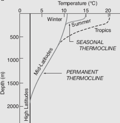
The ocean temperature plays a crucial role in the global climate system, ocean currents and for marine habitats. It varies depending on depth, geographical location and season. Not only does the temperature differ in seawater, so does the salinity. Warm surface water is generally saltier than the cooler deep or polar waters.[1] In polar regions, the upper layers of ocean water are cold and fresh.[2] Deep ocean water is cold, salty water found deep below the surface of Earth's oceans. This water has a uniform temperature of around 0-3 °C.[3] The ocean temperature also depends on the amount of solar radiation falling on its surface. In the tropics, with the Sun nearly overhead, the temperature of the surface layers can rise to over 30 °C (86 °F). Near the poles the temperature in equilibrium with the sea ice is about −2 °C (28 °F).

There is a continuous large-scale circulation of water in the oceans. One part of it is the thermohaline circulation (THC). It is driven by global density gradients created by surface heat and freshwater fluxes.[4][5] Warm surface currents cool as they move away from the tropics. This happens as the water becomes denser and sinks. Changes in temperature and density move the cold water back towards the equator as a deep sea current. Then it eventually wells up again towards the surface.

Ocean temperature as a term applies to the temperature in the ocean at any depth. It can also apply specifically to the ocean temperatures that are not near the surface. In this case it is synonymous with deep ocean temperature).

It is clear that the oceans are warming as a result of climate change and this rate of warming is increasing.[6]: 9 [7] The upper ocean (above 700 m) is warming fastest, but the warming trend extends throughout the ocean. In 2022, the global ocean was the hottest ever recorded by humans.[8]

Definition and types

[edit]

Sea surface temperature

[edit]
Sea surface temperature since 1979 in the extrapolar region (between 60 degrees south and 60 degrees north latitude).[9]
Sea surface temperature (or ocean surface temperature) is the temperature of ocean water close to the surface. The exact meaning of surface varies in the literature and in practice. It is usually between 1 millimetre (0.04 in) and 20 metres (70 ft) below the sea surface. Sea surface temperatures greatly modify air masses in the Earth's atmosphere within a short distance of the shore. The thermohaline circulation has a major impact on average sea surface temperature throughout most of the world's oceans.[10]

Deep ocean temperature

[edit]

Experts refer to the temperature further below the surface as ocean temperature or deep ocean temperature. Ocean temperatures more than 20 metres below the surface vary by region and time. They contribute to variations in ocean heat content and ocean stratification.[11] The increase of both ocean surface temperature and deeper ocean temperature is an important effect of climate change on oceans.[11]

Deep ocean water is the name for cold, salty water found deep below the surface of Earth's oceans. Deep ocean water makes up about 90% of the volume of the oceans. Deep ocean water has a very uniform temperature of around 0-3 °C. Its salinity is about 3.5% or 35 ppt (parts per thousand).[3]

Relevance

[edit]

Ocean temperature and dissolved oxygen concentrations have a big influence on many aspects of the ocean. These two key parameters affect the ocean's primary productivity, the oceanic carbon cycle, nutrient cycles, and marine ecosystems.[12] They work in conjunction with salinity and density to control a range of processes. These include mixing versus stratification, ocean currents and the thermohaline circulation.[citation needed]

Ocean heat content

[edit]

Experts calculate ocean heat content by using ocean temperatures at different depths.

The ocean heat content (OHC) has been increasing for decades as the ocean has been absorbing most of the excess heat resulting from greenhouse gas emissions from human activities.[13] The graph shows OHC calculated to a water depth of 700 and to 2000 meters.

Ocean heat content (OHC) or ocean heat uptake (OHU) is the energy absorbed and stored by oceans.[14] It is an important indicator of global warming.[15] Ocean heat content is calculated by measuring ocean temperature at many different locations and depths, and integrating the areal density of a change in enthalpic energy over an ocean basin or entire ocean.[16]

Between 1971 and 2018, a steady upward trend[17] in ocean heat content accounted for over 90% of Earth's excess energy from global warming.[18][19] Scientists estimate a 1961–2022 warming trend of 0.43 ± 0.08 W/m², accelerating at about 0.15 ± 0.04 W/m² per decade.[20] By 2020, about one third of the added energy had propagated to depths below 700 meters.[21][22] The five highest ocean heat observations to a depth of 2000 meters all occurred in the period 2020–2024.[17] The main driver of this increase has been human-caused greenhouse gas emissions.[23]: 1228 

Measurements

[edit]

There are various ways to measure ocean temperature.[24] Below the sea surface, it is important to refer to the specific depth of measurement as well as measuring the general temperature. The reason is there is a lot of variation with depths. This is especially the case during the day. At this time low wind speed and a lot of sunshine may lead to the formation of a warm layer at the ocean surface and big changes in temperature as you get deeper. Experts call these strong daytime vertical temperature gradients a diurnal thermocline.[25]

The basic technique involves lowering a device to measure temperature and other parameters electronically. This device is called CTD which stands for conductivity, temperature, and depth.[26] It continuously sends the data up to the ship via a conducting cable. This device is usually mounted on a frame that includes water sampling bottles. Since the 2010s autonomous vehicles such as gliders or mini-submersibles have been increasingly available. They carry the same CTD sensors, but operate independently of a research ship.

Scientists can deploy CTD systems from research ships on moorings gliders and even on seals.[27] With research ships they receive data through the conducting cable. For the other methods they use telemetry.

There are other ways of measuring sea surface temperature.[28] At this near-surface layer measurements are possible using thermometers or satellites with spectroscopy. Weather satellites have been available to determine this parameter since 1967. Scientists created the first global composites during 1970.[29]

The Advanced Very High Resolution Radiometer (AVHRR) is widely used to measure sea surface temperature from space.[24]: 90 

There are various devices to measure ocean temperatures at different depths. These include the Nansen bottle, bathythermograph, CTD, or ocean acoustic tomography. Moored and drifting buoys also measure sea surface temperatures. Examples are those deployed by the Global Drifter Program and the National Data Buoy Center. The World Ocean Database Project is the largest database for temperature profiles from all of the world's oceans.[30]

A small test fleet of deep Argo floats aims to extend the measurement capability down to about 6000 meters. It will accurately sample temperature for a majority of the ocean volume once it is in full use.[31][32]

The most frequent measurement technique on ships and buoys is thermistors and mercury thermometers.[24]: 88  Scientists often use mercury thermometers to measure the temperature of surface waters. They can put them in buckets dropped over the side of a ship. To measure deeper temperatures they put them on Nansen bottles.[24]: 88 

Monitoring through Argo program

[edit]
Argo is an international programme for researching the ocean. It uses profiling floats to observe temperature, salinity and currents. Recently it has observed bio-optical properties in the Earth's oceans. It has been operating since the early 2000s. The real-time data it provides support climate and oceanographic research.[33][34] A special research interest is to quantify the ocean heat content (OHC). The Argo fleet consists of almost 4000 drifting "Argo floats" (as profiling floats used by the Argo program are often called) deployed worldwide. Each float weighs 20–30 kg. In most cases probes drift at a depth of 1000 metres. Experts call this the parking depth. Every 10 days, by changing their buoyancy, they dive to a depth of 2000 metres and then move to the sea-surface. As they move they measure conductivity and temperature profiles as well as pressure. Scientists calculate salinity and density from these measurements. Seawater density is important in determining large-scale motions in the ocean.

[citation needed]

Ocean warming

[edit]
The illustration of temperature changes from 1960 to 2019 across each ocean starting at the Southern Ocean around Antarctica.[35]
[edit]

It is clear that the ocean is warming as a result of climate change, and this rate of warming is increasing.[36]: 9  The global ocean was the warmest it had ever been recorded by humans in 2022.[37] This is determined by the ocean heat content, which exceeded the previous 2021 maximum in 2022.[37] The steady rise in ocean temperatures is an unavoidable result of the Earth's energy imbalance, which is primarily caused by rising levels of greenhouse gases.[37] Between pre-industrial times and the 2011–2020 decade, the ocean's surface has heated between 0.68 and 1.01 °C.[38]: 1214 

The majority of ocean heat gain occurs in the Southern Ocean. For example, between the 1950s and the 1980s, the temperature of the Antarctic Southern Ocean rose by 0.17 °C (0.31 °F), nearly twice the rate of the global ocean.[39]

The warming rate varies with depth. The upper ocean (above 700 m) is warming the fastest. At an ocean depth of a thousand metres the warming occurs at a rate of nearly 0.4 °C per century (data from 1981 to 2019).[40]: Figure 5.4  In deeper zones of the ocean (globally speaking), at 2000 metres depth, the warming has been around 0.1 °C per century.[40]: Figure 5.4  The warming pattern is different for the Antarctic Ocean (at 55°S), where the highest warming (0.3 °C per century) has been observed at a depth of 4500 m.[40]: Figure 5.4 

Overall, scientists project that all regions of the oceans will warm by 2050, but models disagree for SST changes expected in the subpolar North Atlantic, the equatorial Pacific, and the Southern Ocean.[41] The future global mean SST increase for the period 1995-2014 to 2081-2100 is 0.86 °C under the most modest greenhouse gas emissions scenarios, and up to 2.89 °C under the most severe emissions scenarios.[41]

A study published in 2025 in Environmental Research Letters reported that global mean sea surface temperature increases had more than quadrupled, from 0.06 K per decade during 1985–89 to 0.27 K per decade for 2019–23.[42] The researchers projected that the increase inferred over the past 40 years would likely be exceeded within the next 20 years.[42]

Causes

[edit]

The cause of recent observed changes is the warming of the Earth due to human-caused emissions of greenhouse gases such as carbon dioxide and methane.[43] Growing concentrations of greenhouse gases increases Earth's energy imbalance, further warming surface temperatures.[8] The ocean takes up most of the added heat in the climate system, raising ocean temperatures.[7]

Main physical effects

[edit]

Increased stratification and lower oxygen levels

[edit]

Higher air temperatures warm the ocean surface. And this leads to greater ocean stratification. Reduced mixing of the ocean layers stabilises warm water near the surface. At the same time it reduces cold, deep water circulation. The reduced up and down mixing reduces the ability of the ocean to absorb heat. This directs a larger fraction of future warming toward the atmosphere and land. Energy available for tropical cyclones and other storms is likely to increase. Nutrients for fish in the upper ocean layers are set to decrease. This is also like to reduce the capacity of the oceans to store carbon.[citation needed]

Warmer water cannot contain as much oxygen as cold water. Increased thermal stratification may reduce the supply of oxygen from the surface waters to deeper waters. This would further decrease the water's oxygen content.[44] This process is called ocean deoxygenation. The ocean has already lost oxygen throughout the water column. Oxygen minimum zones are expanding worldwide.[45]: 471 

Changing ocean currents

[edit]

Varying temperatures associated with sunlight and air temperatures at different latitudes cause ocean currents. Prevailing winds and the different densities of saline and fresh water are another cause of currents. Air tends to be warmed and thus rise near the equator, then cool and thus sink slightly further poleward. Near the poles, cool air sinks, but is warmed and rises as it then travels along the surface equatorward. The sinking and upwelling that occur in lower latitudes, and the driving force of the winds on surface water, mean the ocean currents circulate water throughout the entire sea. Global warming on top of these processes causes changes to currents, especially in the regions where deep water is formed.[46]

In the geologic past

[edit]

Scientists believe the sea temperature was much hotter in the Precambrian period. Such temperature reconstructions derive from oxygen and silicon isotopes from rock samples.[47][48] These reconstructions suggest the ocean had a temperature of 55–85 °C 2,000 to 3,500 million years ago. It then cooled to milder temperatures of between 10 and 40 °C by 1,000 million years ago. Reconstructed proteins from Precambrian organisms also provide evidence that the ancient world was much warmer than today.[49][50]

The Cambrian Explosion approximately 538.8 million years ago was a key event in the evolution of life on Earth. This event took place at a time when scientists believe sea surface temperatures reached about 60 °C.[51] Such high temperatures are above the upper thermal limit of 38 °C for modern marine invertebrates. They preclude a major biological revolution.[52]

During the later Cretaceous period, from 100 to 66 million years ago, average global temperatures reached their highest level in the last 200 million years or so.[53] This was probably the result of the configuration of the continents during this period. It allowed for improved circulation in the oceans. This discouraged the formation of large scale ice sheet.[54]

Data from an oxygen isotope database indicate that there have been seven global warming events during the geologic past. These include the Late Cambrian, Early Triassic, Late Cretaceous, and Paleocene-Eocene transition. The surface of the sea was about 5-30º warmer than today in these warming periods.[12]

See also

[edit]

References

[edit]
Revisions and contributorsEdit on WikipediaRead on Wikipedia
from Grokipedia
Ocean temperature refers to the thermal state of throughout the world's oceans, characterized by significant spatial and vertical gradients driven by solar insolation, ocean circulation, and water's . Globally, the volume-averaged temperature is just above , reflecting the vast extent of cold deep and abyssal waters that constitute over 90% of the ocean's volume, while the mean hovers around 17 °C. Surface temperatures exhibit pronounced latitudinal variation, typically exceeding 25 °C in tropical regions due to intense solar heating and dropping to near -1.8 °C in polar areas where ice formation and of cold deep water prevail. With increasing depth, temperatures decline rapidly across the —a transitional layer where vertical mixing diminishes—stabilizing at 1–4 °C in the deep ocean below approximately 1,000 meters, with minimal seasonal fluctuation owing to isolation from atmospheric influences. These patterns are modulated by currents like the , which transports heat poleward, and phenomena such as El Niño-Southern Oscillation, which can induce basin-wide anomalies exceeding 2 °C. Empirical records, derived from ship measurements, buoys, and floats since the mid-20th century, indicate a long-term rise in sea surface temperatures of about 0.06 °C per decade from 1900 to 2019, with accelerated upper-ocean heat uptake absorbing roughly 90% of Earth's excess radiative imbalance. However, early-20th-century estimates may exhibit a cold bias due to sparse sampling in undersurveyed regions, potentially overstating recent trends upon correction. Oceans' thermal inertia buffers atmospheric variability but amplifies shifts, , and sea-level rise via expansion, underscoring their central role in Earth's climate dynamics.

Fundamental Concepts

Definitions and Classifications

Ocean refers to the thermal state of , quantified in degrees (°C), with global ranges typically from -2°C in polar deep waters to over 30°C in tropical surface layers. This parameter influences water density, circulation, and marine ecosystems through its interaction with and . Measurements distinguish between in-situ temperature, recorded at depth under , and potential temperature, the value the water parcel would attain if adiabatically transported to the sea surface without heat exchange. A more thermodynamically consistent metric, conservative temperature, approximates the per unit mass and differs from potential temperature by up to 1°C in warm, fresh waters but remains within ±0.05°C for most oceanic conditions. Sea surface temperature (SST) specifically denotes the temperature of the ocean's uppermost layer, from the skin (top few millimeters) to depths of up to 20 meters, directly affecting air-sea heat fluxes and atmospheric dynamics. Vertically, temperature exhibits a stratified structure: the surface , where homogenizes temperatures; the , a transitional zone of sharp gradient (often 500–1,000 meters thick) separating warmer surface waters from colder depths; and the deep , where temperatures stabilize near 0–4°C with minimal variation. The 's depth and intensity vary seasonally and latitudinally, deepening in and shoaling in mid-latitudes during summer. Ocean waters are classified into water masses based on characteristic temperature-salinity (T-S) signatures acquired during formation in source regions, enabling identification via T-S diagrams. These include surface waters like subtropical mode waters (warm, saline), intermediate waters such as Antarctic Intermediate Water (cooler, fresher), and deep waters like (around 2–4°C, high salinity) or (near -0.5°C, oxygen-rich). Such classifications trace pathways, as water masses conserve their properties adiabatically until mixing occurs. Horizontally, temperatures are zoned by , with equatorial bands exceeding 25°C, subtropical gyres around 15–20°C, and polar regions below 5°C, modulated by currents and .

Thermodynamic Role in Climate System

Water's of approximately 4.18 J/g·°C enables the oceans to store vast amounts of with minimal temperature fluctuations, far exceeding the atmosphere's capacity of about 1.0 J/g·°C for dry air. Seawater's effective , around 3,900 J/kg·°C, combined with the oceans' volume—covering 71% of Earth's surface and extending to average depths of 3,700 meters—results in the ocean holding roughly 1,000 times the of the entire atmosphere. This thermodynamic property positions the oceans as the primary heat reservoir in the , absorbing solar radiation and modulating global energy distribution. Since the mid-20th century, oceans have sequestered over 90% of excess heat from anthropogenic , with reaching record levels by 2023. This uptake, quantified through integrated measurements to depths of 2,000 meters, buffers rises but drives contributing to increase. The ocean's thermal inertia delays full climate responses to , stabilizing short-term variability while amplifying long-term changes through feedbacks like altered circulation. Ocean currents, propelled by density gradients from and variations, transport poleward at rates up to 1 petawatt in the Atlantic, reducing equator-to-pole contrasts that would otherwise prevail under atmospheric transport alone. The , including components like the Atlantic Meridional Overturning Circulation, redistributes this vertically and horizontally, influencing regional s and patterns such as Hadley cells. Surface ocean s also regulate and fluxes to the atmosphere, fueling phenomena like monsoons and hurricanes while exerting a effect that tempers extreme warming in tropical regions. Disruptions to these dynamics, such as from freshwater influx, could weaken transport and exacerbate .

Observation Methods

Historical Approaches

Early observations of ocean temperature focused on (SST), with systematic measurements commencing in the late using mercury thermometers inserted into water samples hauled aboard ships via buckets or directly suspended overboard. These initial efforts, driven by scientific curiosity rather than routine monitoring, provided sparse data primarily from exploratory voyages. By the , the bucket method became standardized, involving wooden or receptacles lowered to the sea surface, filled with , and then measured promptly with unprotected or protected mercury thermometers to minimize exposure time and evaporative cooling biases. Wooden buckets, common until the early , induced greater temperature depression (up to 0.5–1°C) due to slower hauling and higher heat loss compared to later or uninsulated rubber variants. expanded through and naval logs, such as those from the British Royal Navy and ships, yielding datasets like the International Comprehensive Ocean-Atmosphere Data Set (ICOADS) precursors with coverage increasing from fewer than 1,000 observations annually in 1850 to over 100,000 by 1900. Subsurface temperature profiling emerged in the late with the development of reversing thermometers by François-Alphonse Forel in 1877 and their integration into Nansen bottles by around 1900, allowing protected deep-water samples to be isolated at depth and measured upon retrieval without pressure distortion. These mechanical samplers, deployed via hydrographic casts, enabled vertical profiles to depths of several thousand meters, though resolution remained coarse (typically 10–20 depths per cast) and labor-intensive, limiting frequency to dedicated expeditions like the 1872–1876 Challenger voyage, which recorded over 350 stations. From the 1930s onward, shipboard methods evolved with the adoption of engine-room intake thermometers, which sampled water piped for cooling at 2–10 meters depth, reducing bucket-related artifacts but introducing hull-induced warming biases of 0.2–0.5°C; this transition coincided with expansions in naval observations. Auxiliary techniques included mechanical bathythermographs (MBTs) from the 1930s, which traced shallow profiles (to 200–300 meters) via towed or lowered probes, and early radiation thermometers for non-contact SST estimates, though these were sporadic until post-1940s refinements. Overall, pre-1950 records suffered from inhomogeneous coverage, with biases and seasonal gaps, necessitating subsequent adjustments for instrument and platform shifts to reconstruct reliable baselines.

Modern Instrumentation and Satellites

Modern satellite observations of (SST) primarily utilize infrared radiometers and sensors to infer skin-layer temperatures from thermal emissions, with corrections for atmospheric effects such as and aerosols. The Advanced Very High Resolution Radiometer (AVHRR), operational on NOAA polar-orbiting satellites since the late 1970s and continued on platforms like MetOp-A/B/C, provides global SST data at spatial resolutions of approximately 1 km, aggregated into daily 0.25° grid products with accuracies around 0.02 against buoy validations, though standard deviations reach 0.25 K due to contamination and diurnal variability. Blended analyses, such as NOAA's Optimum SST (OISST), integrate AVHRR with data from instruments like the Advanced Microwave Scanning Radiometer-EOS (AMSR-E) on Aqua (launched 2002) to mitigate biases, achieving near-daily global coverage between 60°S and 60°N. Subsurface temperature profiling relies on autonomous platforms, notably the array, which deploys over 3,900 profiling floats globally since full implementation around 2004, following initial deployments in 1999. These neutrally buoyant floats drift at depth, ascend to the surface every 10 days to measure and profiles from 2,000 m to the surface using embedded conductivity--depth (CTD) sensors, providing unprecedented three-dimensional coverage of the upper ocean with vertical resolutions of 10-20 m and uncertainties typically below 0.002°C for . Argo data, disseminated in near real-time, cover ice-free regions poleward to about 80° latitude, enabling quantification of heat content anomalies with basin-scale precision. Complementary instrumentation includes shipborne CTD rosettes, which deploy sensor s to sample full-depth profiles with accuracies of 0.001°C for via resistance thermometers, often integrated with oxygen and bio-optical sensors for contextual validation. Autonomous underwater gliders, equipped with miniaturized CTDs (e.g., 1-2 mm diameter sensors), execute sawtooth dives to 1,000 m or more, yielding hourly profiles over missions lasting weeks to months, with temperature precisions around 0.002°C, enhancing spatial sampling in dynamic regions like coastal zones. Moored buoys, such as those in NOAA's Tropical Atmosphere array, provide time-series measurements at fixed depths using ruggedized CTDs, logging data at intervals of minutes to hours with minimal drift over multi-year deployments. These systems collectively address satellite limitations in subsurface access and polar/near-coastal gaps, though against in-situ references remains essential to counter sensor and instrumental biases.

Data Quality Assessments

In situ sea surface temperature (SST) measurements face multiple sources of uncertainty, including instrumental errors, sampling biases, and environmental factors such as sensor exposure to air or deck heating. A comprehensive identifies key components: random measurement errors (typically 0.1–0.5°C for historical buckets), systematic biases from method transitions (e.g., uninsulated to insulated buckets or ship engine intakes), and spatial leading to uncertainties. These contribute to overall SST dataset uncertainties of approximately 0.1°C for global means in recent decades, escalating to 0.2–0.5°C in the early due to sparse coverage and unadjusted cooling biases from canvas bucket . Homogenization adjustments aim to correct for these inhomogeneities but introduce their own uncertainties, often comparable to observed decadal variability. For instance, datasets like HadSST and ERSST apply time-dependent bias corrections for types and depths, yet unresolved differences persist across products, with early-20th-century SSTs potentially underestimated by 0.2–0.4°C due to inadequate canvas insulation modeling. Independent analyses using instrumentally homogeneous subsets confirm post-1950 warming trends of 0.07–0.1°C per decade but highlight larger (up to 0.3°C) before 1940 from uncorrected wartime disruptions and measurement practice shifts. Subsurface temperature data from floats undergo rigorous real-time and delayed-mode to flag outliers, spikes, and drifts, with typical single-measurement accuracies of 0.002°C after corrections for response times and lags. However, systematic issues like conductivity cell fouling or drifts can propagate to temperature via salinity-derived effects, necessitating expert adjustments in delayed-mode processing; uncorrected floats may exhibit biases up to 0.01°C in deep profiles. Coverage remains uneven in polar regions and marginal seas, amplifying gridding uncertainties in global products. Ocean heat content (OHC) estimates integrate these temperature profiles with depth-dependent uncertainties, historically inflated by expendable (XBT) fall-rate biases (up to 10% depth errors) and sparse sampling pre-. Modern assessments quantify OHC uncertainties at 0.5–1.0 × 10^{22} J for upper 2000 m since 2005, driven by profile-to-grid mapping and end-member assumptions in objective analyses, though has reduced them by an compared to 1970s-era ship casts. The International Quality-controlled Ocean Database (IQuOD) standardizes flags and uncertainty propagation across profiles, revealing that deep-ocean (>2000 m) trends carry higher relative errors (0.1–0.5°C per century) due to limited observations and model-derived interpolations.

Patterns of Variability

Spatial Gradients and Zonation

Ocean temperature displays marked spatial gradients horizontally across and vertically through depth, delineating distinct thermal zonations that influence circulation, ecosystems, and heat transport. The dominant horizontal gradient is latitudinal, with sea surface temperatures (SSTs) averaging 25–30°C near the —peaking around 28–29°C in the western equatorial Pacific—and declining poleward to approximately -1.8°C in polar regions, reflecting the cosine variation in solar insolation with latitude. This equator-to-pole SST contrast, typically 25–30°C globally, steepens in winter hemispheres due to seasonal cooling and is modulated by ocean currents; for instance, the elevates mid-latitude North Atlantic SSTs by 5–10°C relative to zonal averages. In the , the gradient is more symmetric and pronounced owing to the encircling , whereas landmasses introduce longitudinal asymmetries, such as cooler eastern boundaries from . Vertically, the ocean stratifies into three primary thermal zones: the surface (0–50 to 200 m depth, depending on and ), where temperatures align closely with SSTs and uniformity prevails due to wind-driven mixing; the (often 100–1000 m), characterized by a sharp gradient of 0.01–0.1°C per meter dropping from ~20°C to 5–10°C; and the deep ocean below (~1000 m to abyss), maintaining near-uniform temperatures of 1–4°C with gradients under 0.001°C/m, as adiabatic compression and homogenize heat. depth and intensity vary zonally: in tropical oceans, a permanent resides at 100–200 m, enabling efficient heat trapping; subtropical gyres deepen it to 500–1000 m with weaker gradients; polar regions feature seasonal absence of a distinct , with winter mixing to 500–1000 m depths, erasing gradients until summer restratification. These vertical zonations arise from surface heating, , and effects on , with the 20°C isotherm often defining the base in equatorial profiles. Horizontal zonation beyond latitude includes coastal-offshore and frontal structures; eastern boundary upwelling zones, like or currents, sustain 5–15°C cooler SSTs than adjacent open due to lifting cold deep water, forming persistent thermal fronts with gradients exceeding 1°C/km. Conversely, western boundary currents such as the Kuroshio or Current intensify warm gradients, transporting equatorial heat poleward at rates enhancing meridional by factors of 2–5 over diffusive estimates. Subtropical gyre interiors exhibit subdued gradients, with SSTs 1–3°C warmer than gyre edges from downwelling suppression of mixing. These patterns, verifiable via floats and altimetry, underscore causal roles of Coriolis effects, wind stress curl, and forcing in shaping thermal zonation, independent of long-term trends.

Temporal Fluctuations and Cycles

Ocean surface temperatures exhibit diurnal fluctuations, with daytime solar heating raising sea surface temperatures (SSTs) by up to 1-2°C in low-wind conditions over the , while nocturnal cooling restores equilibrium through longwave radiation and . These short-term variations are most pronounced in calm, shallow coastal waters and diminish with depth or during stormy periods that enhance vertical mixing. Seasonal cycles dominate temporal variability in SSTs, driven primarily by latitudinal differences in insolation and the annual migration of the sun. In mid-latitudes, SST amplitudes reach 10-15°C between summer maxima and winter minima, reflecting shallow mixed layers that allow rapid response to atmospheric forcing. Tropical oceans show smaller amplitudes of 1-3°C due to persistent stratification and weaker seasonal insolation contrasts. Globally, the SST seasonal cycle has intensified by approximately 3.9% from 1983 to 2022, with amplified warming in northern mid-latitudes linked to reduced and altered heat fluxes. On interannual timescales, the El Niño-Southern Oscillation (ENSO) imposes the strongest fluctuations, with El Niño events elevating equatorial Pacific SSTs by 2-3°C in the Niño 3.4 region (5°S-5°N, 120°-170°W) for 6-18 months, while La Niña phases cool the same area by similar magnitudes. These anomalies propagate globally via atmospheric teleconnections, contributing up to 20-30% of year-to-year SST variance outside the Pacific. ENSO's irregular cycle, averaging 2-7 years, modulates tropical cyclone activity and drought patterns through altered . Decadal and multidecadal oscillations further structure longer-term fluctuations. The (PDO), identified in North Pacific SSTs poleward of 20°N, features warm phases enhancing Aleutian Low intensity and cool phases suppressing it, with indices fluctuating on 20-30 year timescales and amplitudes of 0.5-1°C in regional means. Similarly, the Atlantic Multidecadal Oscillation (AMO) manifests as basin-wide North Atlantic SST variations of 0.4°C over 60-80 year periods, influencing rainfall and hurricane frequency. However, analyses of extended instrumental records question the oscillatory nature of PDO and AMO, attributing much of their signal to variability or external forcing rather than intrinsic cycles.

Historical Records

Paleoceanographic Proxies

Paleoceanographic proxies reconstruct past ocean temperatures from geological records, including marine sediments, corals, and speleothems, extending instrumental data back millions of years. These methods rely on empirical calibrations linking geochemical or biological signals in archives to modern temperature analogs, enabling quantification of sea surface temperatures (SSTs), subsurface conditions, and deep-water masses. Proxies are categorized as inorganic (e.g., isotope and trace element ratios in carbonates) or organic (e.g., lipid biomarkers), with multiproxy syntheses used to mitigate individual uncertainties such as diagenesis, vital effects, or environmental confounders. Reconstructions reveal glacial-interglacial SST swings of 4–8°C in many basins and warmer Eocene oceans exceeding 30°C equatorially. Oxygen ratios (δ¹⁸O) in planktic and benthic foraminiferal serve as a foundational proxy, where lighter δ¹⁸O incorporation increases with cooler temperatures at roughly -0.22‰ per °C due to thermodynamic . Planktic like Globigerinoides ruber record upper SSTs, while benthic forms such as Cibicides wuellerstorfi track deep-sea temperatures below 2–4°C in modern oceans. However, δ¹⁸O signals confound temperature with seawater δ¹⁸O variations from salinity gradients or global ice volume, which can amplify apparent cooling by 1–2‰ during Pleistocene glacials; paired proxies often disentangle these. This method has underpinned records spanning the , though spatial biases favor low-latitude data and assume constant factors. Magnesium-to-calcium ratios (Mg/Ca) in foraminiferal tests provide a complementary , as Mg substitution in rises exponentially with (calibrated as Mg/Ca = 0.38 exp(0.090 T) mmol/mol for some , yielding SSTs from core-tops matching modern values within 1–2°C). This proxy isolates temperature from δ¹⁸Osw effects, facilitating ice-volume-independent deep-ocean reconstructions, such as Miocene cooling trends. Planktic Mg/Ca targets SSTs (e.g., 22–26°C in Early Cretaceous neritic settings), while benthic applications reveal bottom-water stability. Limitations include species-specific "vital effects" (±1–2°C offsets), dissolution in undersaturated waters reducing Mg/Ca by up to 10–20%, and salinity influences requiring corrections; dissolution-adjusted calibrations improve accuracy for pre-Quaternary records. Organic proxies like the alkenone unsaturation index (Uᴷ'₃₇ = [C₃₇:₂]/[C₃₇:₂ + C₃₇:₃]) from correlate linearly with SSTs (Uᴷ'₃₇ = 0.033 T - 0.044, valid 0–30°C), preserving signals in sediments with minimal alteration. This reconstructs SSTs aligning with foraminiferal data within 1°C and indicates in past climates. Regional calibrations address non-temperature factors like growth season or nutrient stress, enhancing fidelity in high-latitude or zones. The TEX₈₆ index, derived from glycerol dialkyl glycerol tetraethers (GDGTs) of marine Thaumarchaeota, measures cyclization degrees reflecting upper-ocean temperatures (SST = 33.4 - 32.8 TEX₈₆ for global calibration, accurate to ±2–3°C in ). It excels in organic-rich sediments for SSTs, capturing subsurface signals up to 200 m depth, but exhibits regional warm biases (e.g., +4–6°C in ) and potential or oxygen influences confounding signals. Multiproxy comparisons, such as TEX₈₆ with Uᴷ'₃₇, validate records while highlighting discrepancies from export productivity or archaeal . Coral Sr/Ca ratios and clumped isotopes (Δ₄₇) offer high-resolution proxies for tropical SSTs over Holocene timescales, with Sr/Ca decreasing ~0.05 mmol/mol per °C and Δ₄₇ independent of δ¹⁸Osw. These extend to reef archives but are limited by upwelling or dissolution. Overall, proxy ensembles, stack-averaged for global means, indicate Phanerozoic ocean warmth exceeding modern levels by 5–10°C during greenhouse intervals, with uncertainties shrinking via Bayesian frameworks.

Instrumental Observations from 1850 Onward

Instrumental records of ocean temperature from 1850 onward rely predominantly on sea surface temperature (SST) measurements collected via ships, with subsurface data emerging later and remaining sparse until the mid-20th century. The International Comprehensive Ocean-Atmosphere Data Set (ICOADS) serves as the foundational archive, compiling over 500 million marine observations from 1662 to present, though systematic SST coverage intensifies after 1850 along major shipping lanes. Early SST determinations used thermometers inserted into water samples hauled aboard in canvas or wooden buckets, a method prone to underestimation due to evaporative cooling and exposure to deck air temperatures 1–2°C below the sea surface. By the early 20th century, engine-room intake measurements supplemented bucket samples on steamships, reducing some biases but introducing others related to intake depth and flow dynamics. Gridded SST products derived from ICOADS, such as HadSST.4 and Extended Reconstructed SST (ERSST) version 6, apply bias corrections for these historical methods, including adjustments for bucket type (canvas cooling by ~0.2–0.5°C versus wooden) and ship metadata like speed and hull material. HadSST.4, spanning 1850–2018, employs an ensemble approach to quantify uncertainties, revealing higher variability in pre-1900 estimates due to limited observations. ERSST incorporates data post-1970s and floats for validation, showing closer alignment with independent profile data than earlier versions. Intercomparisons indicate differences of up to 0.3°C in regional SST anomalies before 1950 between HadSST and ERSST, stemming from varying homogenization techniques and infilling of sparse grids via . Coverage gaps persist in the and polar regions through the 19th and early 20th centuries, with observations concentrated in the North Atlantic and Pacific trade routes, leading to extrapolated estimates with uncertainties exceeding 0.5°C in under-sampled areas. Recent analyses suggest early-20th-century SSTs (1900–1930) may have been overestimated as cooler by 0.2–0.4°C in prior reconstructions due to unaccounted shifts in measurement practices during . Subsurface ocean temperature observations began sporadically in the late via reversing thermometers on Nansen bottles during oceanographic expeditions, but reliable profiles with near-global coverage only emerged from the late using mechanical bathythermographs (MBTs) deployed from ships. These devices measured temperatures to depths of 200–300 meters, though sampling remained irregular and biased toward military routes until the . Datasets like EN4 provide subsurface profiles from 1900 onward, but pre-1950 data are limited to upper 700 meters in select basins, with quality controls addressing instrument calibration drifts of up to 0.1°C per decade. Instrumental homogeneity improved post-1970 with expendable bathythermographs (XBTs), which extended profiles to 750 meters but required corrections for fall-rate errors causing depth overestimation by 1–5% in early deployments. From the 1980s, moored buoys (e.g., Tropical Atmosphere Ocean array) and drifting buoys augmented ship data, enhancing to ~0.25°C in tropical bands by the . The program, deploying autonomous floats since 2000, delivers over 400,000 upper-ocean (to 2,000 meters) profiles annually, reducing uncertainties to ~0.002°C for global averages through redundant sensors and real-time quality checks. Despite these advances, unresolved biases in historical adjustments—such as potential over-cooling in WWII-era engine intakes—contribute to uncertainties in decadal-scale variability, with some analyses indicating amplified trends in adjusted datasets relative to raw observations. Overall, instrumental records document a transition from regionally sparse SST proxies to vertically resolved, near-global monitoring, though pre-1950 data retain elevated error margins due to methodological inconsistencies.

20th-Century Changes

Global s (SST) exhibited a net warming of approximately 0.6°C over the , based on analyses of historical instrumental records compiled in datasets such as HadSST4 and NOAA's Extended Reconstructed SST (ERSST). This estimate derives from monthly gridded anomalies relative to a 1961–1990 baseline, incorporating ship-based measurements, which dominated early records, and later buoy data. The rate averaged about 0.06°C per decade from 1900 to 2000, though with significant decadal variability. The warming displayed distinct phases: a pronounced increase of roughly 0.3–0.4°C from 1900 to the early 1940s, driven partly by natural variability including the Atlantic Multidecadal Oscillation; a subsequent period of stagnation or mild cooling (approximately -0.1°C) from the 1940s to the mid-1970s, influenced by emissions and internal ocean-atmosphere oscillations; and accelerated warming post-1975 aligning with the latter half of the century's net trend. These patterns are evident in multiple reconstructions, though regional differences were notable, with stronger warming in the oceans compared to the Southern. Uncertainties persist due to sparse early sampling, primarily from voluntary observing ships, and systematic biases in measurement methods, such as underestimation from uninsulated bucket thermometers leading to a cold bias of up to 0.5°C in early 20th-century estimates. Correcting for such biases reduces the implied 1900–1950 warming by 20–50%, suggesting standard datasets may overestimate the century's net SST rise. Subsurface ocean temperatures, inferred from later Argo floats and historical profiles, indicate heat accumulation in the upper 700 meters consistent with surface trends, though full-depth assessments for the early century remain limited. These adjustments highlight challenges in attributing changes solely to external forcings amid natural variability.

21st-Century Accelerations and Records

Global sea surface temperatures (SST) have exhibited accelerated warming trends since the early 2000s, with peer-reviewed analyses indicating a statistically significant increase in the rate of ocean heat uptake. From 1961 to 2022, ocean warming accelerated at a rate of 0.15 ± 0.04 W m⁻² per decade, contributing to a total warming of 0.43 ± 0.08 W m⁻² over the period. This acceleration is linked to rising Earth's energy imbalance, manifesting as faster multidecadal SST increases detectable in satellite and in-situ observations. Since the , global ocean warming has intensified by over 25%, driven by enhanced heat accumulation in mode and intermediate waters. Upper (OHC), a direct measure of integrated changes, has risen steadily from onward, with the top 2000 meters absorbing approximately 90% of excess planetary . Annual OHC anomalies for 0-2000 m show consistent positive trends through 2024, surpassing prior decades in magnitude. In the 2010-2019 decade, surface warming rates reached 0.280 ± 0.068°C per decade, over four times the long-term average, reflecting deeper penetration of into the ocean profile. Record highs have been repeatedly set in the , culminating in 2023 and 2024. On August 22, 2023, global average daily SST peaked at 18.99°C (66.18°F), the highest in observational records. The year 2024 marked the warmest ocean on record, with both SST and upper 2000 m OHC achieving unprecedented levels, exceeding 2023 benchmarks. This 2023-2024 SST jump exceeded prior records by at least 0.25°C globally and 0.42°C in the North Atlantic, an event deemed low-probability under historical trends but consistent with ongoing heat accumulation. These records align with broader surface temperature anomalies, where 2024's global ocean surface reached 1.15°C above the 20th-century average.

Ocean Heat Content Dynamics

Ocean heat content (OHC) quantifies the total stored in the ocean, computed as the integral of temperature anomalies weighted by , , and volume over specified depth ranges and global extents, typically expressed in zettajoules (10^21 J). This metric captures subsurface heat storage beyond surface temperatures, revealing that approximately 91% of excess energy trapped by greenhouse gases has been absorbed by the oceans since the mid-20th century. Empirical estimates indicate a net OHC increase of about 436 zettajoules from 1971 to 2018, with the upper 2000 meters accounting for the majority of this accumulation due to limited deep-ocean mixing. Dynamics of OHC involve surface heat fluxes from the atmosphere—primarily longwave radiation, latent, and —followed by downward transport via turbulent , mixing, and large-scale circulation patterns such as the meridional overturning circulation. Ocean heat uptake efficiency, defined as the ratio of oceanic heat gain to global surface air temperature rise, has risen by roughly 20% since 1970, potentially linked to enhanced ventilation in subtropical gyres and mode water subduction. Observations from the float array, deployed globally since 2004, have reduced sampling uncertainties to below 0.1 W/m² for full-depth estimates, enabling detection of interannual variability tied to modes like the El Niño-Southern Oscillation, which modulates equatorial heat redistribution. Recent analyses reveal accelerations in OHC accumulation, with rates doubling from pre-1990s levels to approximately 1.0 W/m² during 2010–2022, attributed partly to internal modes favoring enhanced uptake and reduced Atlantic export. However, pre-Argo era data (before 2004) carry larger uncertainties from sparse ship-based measurements and eXpendable (XBT) biases, estimated at up to 20% for upper-ocean trends, necessitating cautious attribution of long-term dynamics. Full-depth OHC reached record levels in 2022, exceeding prior maxima by 14 zettajoules relative to 2021, underscoring the ocean's role as a primary amid ongoing imbalance. Vertical partitioning shows ~75% of gain confined to the upper 700 meters, with slower penetration to abyssal layers via diapycnal mixing rates of order 10^{-5} m²/s. These dynamics imply lagged feedbacks, including contributing ~30% to global sea-level rise since 1993.

Driving Mechanisms

Natural Forcings and Internal Variability

Natural forcings influencing ocean temperatures include variations in , volcanic aerosol injections, and long-term orbital parameters known as . Solar variability, such as the 11-year sunspot cycle, modulates incoming solar radiation by approximately 0.1% globally, leading to small but detectable (SST) responses of about 0.1–0.2°C in the tropical Pacific over decadal scales. Volcanic eruptions, particularly large stratospheric events like the 1991 eruption, inject sulfate aerosols that reflect sunlight, causing global SST cooling of 0.2–0.5°C for 1–3 years post-eruption by reducing surface insolation and enhancing ocean heat uptake. Increased volcanic activity from 2003–2012, including eruptions like (1982) and others, contributed to a temporary reduction in the global warming trend by approximately 0.08°C over that decade through aerosol-induced . Milankovitch cycles—eccentricity (100,000-year period), obliquity (41,000 years), and precession (23,000 years)—alter seasonal insolation distribution by up to 25% at high latitudes, driving long-term ocean temperature oscillations tied to glacial-interglacial transitions, with evidence from deep-sea sediment proxies showing amplified deep-ocean warming during interglacials. Internal variability arises from chaotic interactions within the , producing quasi-oscillatory patterns in ocean temperatures without external forcing. The El Niño-Southern Oscillation (ENSO), with a 2–7 year periodicity, features SST anomalies exceeding 1°C in the equatorial Pacific, where El Niño phases warm global averages by 0.1–0.2°C temporarily via altered and heat redistribution. The (PDO), operating on 20–30 year timescales, manifests as ENSO-like SST patterns north of 20°N, with cool phases enhancing Aleutian Low intensity and contributing to multidecadal cooling in the North Pacific SST by up to 0.5°C. Similarly, the Atlantic Multidecadal Oscillation (AMO) drives North Atlantic SST fluctuations of 0.4–0.5°C over 60–80 years, linked to variations, influencing hemispheric temperature variance and masking forced trends. These modes interact; for instance, PDO and AMO phases can modulate ENSO amplitude, amplifying internal variability's role in regional changes by 20–50% on decadal scales. Attribution studies indicate that while natural forcings dominate paleoclimate variability, internal modes explain much of the interannual-to-decadal fluctuations in modern instrumental records, complicating signal detection amid low-frequency trends. For example, a shift to positive PDO and AMO phases in the mid-20th century contributed to accelerated North Pacific and Atlantic warming, independent of radiative changes. Ocean circulation, such as propagation, further propagates these variabilities, with models showing internal ocean dynamics accounting for up to 30% of upper-ocean temperature variance in the extratropics.

Anthropogenic Contributions

Human emissions of greenhouse gases, primarily carbon dioxide from fossil fuel combustion, cement production, and land-use changes, have elevated atmospheric CO₂ concentrations from approximately 280 ppm in the pre-industrial era to over 420 ppm by 2023, enhancing the greenhouse effect and creating a top-of-atmosphere radiative imbalance of about 0.9 W/m². This excess energy, equivalent to roughly 436 zettajoules absorbed by the oceans in the upper 2000 meters from 1971 to 2010, drives ocean warming as the ocean takes up over 90% of the anthropogenic heat excess in the Earth system, buffering atmospheric temperature rise. Attribution analyses, employing detection and attribution techniques that compare observed trends with simulations under anthropogenic and natural forcings, indicate that the post-1950s warming in the global ocean, particularly the subsurface layers, is inconsistent with internal variability or natural drivers like and volcanic aerosols alone. For instance, the observed increase in since the 1970s aligns closely with model projections forced by rising concentrations, with the anthropogenic signal emerging robustly by the late 20th century. Other anthropogenic factors, such as tropospheric from industrial emissions exerting a cooling influence via and brightening, have partially offset warming until recent decades when aerosol regulations reduced their net effect, allowing accelerated heat uptake. However, the dominant driver remains the long-lived es, with their exceeding that of short-lived pollutants. Peer-reviewed studies confirm that without human emissions, recent marine heatwaves and sustained rises, such as those exceeding 1°C in parts of the tropical s since 1900, would be virtually impossible under natural conditions alone.

Challenges in Causal Attribution

Attributing observed changes in ocean temperature to specific causes, particularly anthropogenic greenhouse gas emissions versus natural variability, faces significant methodological hurdles due to the complexity of ocean-atmosphere interactions and limitations in observational data. Causal attribution typically relies on detection and attribution (D&A) frameworks, which compare observed trends against model simulations of natural-only forcings (e.g., , volcanic aerosols) and all-forcings scenarios including anthropogenic factors. However, these approaches struggle to disentangle signals because natural internal variability, such as the Atlantic Multidecadal Oscillation (AMO) or (PDO), operates on decadal to multidecadal timescales that overlap with anthropogenic warming trends, potentially amplifying or masking forced responses. For instance, multidecadal variations in and ocean surface temperature since 1866 are largely attributable to anthropogenic forcing in some analyses, yet interannual and decadal fluctuations remain dominated by natural modes, complicating precise quantification. A primary challenge stems from uncertainties in historical (OHC) measurements, which underpin much of the attribution evidence. Pre-2005 data, before the widespread deployment of the float array, depend on sparse ship-based and moored observations, leading to potential biases in vertical and spatial sampling; for example, global OHC showed no robust trend from 1960 to 1990 due to deep ocean cooling offsetting minor upper-ocean gains, a not fully captured in early reconstructions. Modern estimates indicate the ocean absorbs about 90-91% of excess heat from greenhouse gases, but sensitivity analyses reveal that choices in bias corrections, instrumental errors, and mapping methods can alter decadal OHC trends by factors of 2-3, with upper-ocean (0-700 m) uncertainties exceeding 20% in some periods. These gaps hinder confident separation of effects from unforced variability, as internal ocean modes like meridional overturning circulation can redistribute heat without net surface warming. Climate models introduce further attribution difficulties, as they often underestimate observed internal variability or fail to reproduce spatial patterns of warming. Anthropogenic forcing is expected to produce relatively uniform heat uptake, yet post-2005 OHC increases have concentrated in mid-latitude bands near 40°N and 40°S with minimal tropical or deep-ocean penetration, a more aligned with natural circulation shifts than pure radiative imbalance in some critiques. Detection methods assume model fidelity in simulating counterfactual worlds, but discrepancies—such as early-20th-century cold biases in sea surface temperatures unexplainable by internal variability alone—suggest models may overestimate anthropogenic signals by underweighting unforced land-ocean contrasts. Moreover, attribution of recent accelerations (e.g., post-2010) to reduced cooling versus emerging natural cycles like a potential AMO downturn remains unresolved, as ensemble simulations exhibit wide spread in projected responses. Empirical challenges also arise from confounding factors like volcanic influences and solar cycles, which can induce transient cooling or warming that mimics long-term trends; for example, the 1960-1990 OHC stasis aligns with post-eruption deep cooling rather than a pure anthropogenic pause. Peer-reviewed critiques highlight that while fingerprinting techniques attribute over 70-90% of post-1950 OHC rise to human forcings in optimized models, alternative reconstructions emphasizing decadal rivals question dominance claims, especially regionally. These issues underscore the need for improved observing systems and hybrid statistical-dynamical methods to enhance causal realism, as over-reliance on model-dependent attribution risks conflating correlation with causation amid persistent data voids in the deep ocean (>2000 m), where heat storage uncertainties exceed 50%.

Impacts and Consequences

Physical and Dynamical Effects

Ocean warming induces of seawater, contributing significantly to global mean . Since the 1970s, has accounted for about 30-50% of observed , with estimates indicating it comprised 56% in recent decades as increased. This effect arises from the volumetric expansion of water as it absorbs excess heat, primarily in the upper ocean layers, exacerbating coastal inundation and risks. Increased ocean temperatures enhance upper-ocean stratification by warming surface waters and reducing their relative to deeper layers, which suppresses vertical mixing and entrainment from below. Observations show summertime increases in pycnocline stratification and shallower mixed-layer depths, particularly in subtropical regions, limiting to deeper oceans and amplifying surface warming feedbacks. This stratification intensifies since the mid-20th century, as the ocean has absorbed over 90% of anthropogenic excess heat, altering the gradient and potentially reducing the efficiency of mode water formation. Warmer temperatures disrupt large-scale ocean circulation patterns, including the , by freshening and warming high-latitude surface waters, which stabilizes the water column and weakens overturning. Recent accelerations in ocean heat uptake, nearly doubling since the , have concentrated warming in mid-latitude bands around 40°N and 40°S, influencing gyre dynamics and meridional heat transport. In eastern boundary systems, warming may intensify stratification, shoal upwelling fronts, and alter source water depths, potentially reducing nutrient supply despite stronger winds. These dynamical shifts contribute to regional anomalies, such as delayed upwelling onset in systems like the California Current, where increased stratification traps heat near the surface and modifies cross-shelf exchanges. Overall, ocean heat accumulation since 2005 has focused in specific latitudinal bands with minimal net warming in equatorial zones, reflecting interplay between advection, diffusion, and wind-driven dynamics. Such changes pose challenges for predicting circulation stability, as enhanced hydrological cycles from warming further promote stratification and modulate heat uptake efficiency.

Ecological and Biological Responses

Rising ocean temperatures induce physiological stress in marine organisms, elevating metabolic rates and oxygen demands, which can exceed supply in warmer, less oxygenated waters. Empirical studies document exponential increases in metabolic rates for many aquatic species with temperature rises, leading to heightened during extremes. This metabolic acceleration, observed across taxa including and , amplifies energy requirements by up to several-fold per degree , straining aerobic scopes and contributing to reduced growth and survival under sustained warming. Coral reefs exhibit acute sensitivity, with bleaching events triggered by seawater anomalies of 1–2°C above seasonal norms, causing symbiotic algae expulsion and potential colony mortality. The fourth global coral bleaching event, confirmed in 2024, affected reefs across the Atlantic, Pacific, and Indian Oceans, following prior episodes in 1998, 2010, and 2014–2017, correlating with marine heatwaves and record sea surface temperatures. From 2023 to September 2025, bleaching-level heat stress impacted 84.4% of global reef area, with mass bleaching in over 62% of monitored sites, though recovery varies by region and species resilience. Warmer conditions exacerbate irradiance stress, reducing and in surviving corals. Marine species distributions have shifted poleward or to deeper habitats in response to warming, with over half of tracked populations relocating toward cooler latitudes. Along U.S. coasts, empirical data from fisheries surveys indicate northward expansions averaging 72 km per decade for demersal species since the , driven by thermal tolerance limits. In the , warming facilitates influx of subtropical species into polar ecosystems, altering community structures. These migrations disrupt predator-prey synchrony, as evidenced by mismatched in migratory species like whales and seabirds, where warming alters spawning and timings by weeks to months. Fisheries productivity reflects these biotic rearrangements, with historical warming linked to a 3–4% decline in global maximum catch potential since , particularly in tropical regions where thermal optima are exceeded. Peer-reviewed analyses of 232 project further reductions of up to 30% by 2050 under moderate emissions, compounded by range contractions and failures in overfished populations. Conversely, temperate and polar fisheries may see transient gains from influxes, such as tropicalization enhancing herbivory in forests, though cascading effects like habitat loss from heatwaves often offset benefits. Planktonic communities, foundational to food webs, show variable responses; warming enhances stratification, reducing nutrient upwelling and in some gyres, while empirical experiments indicate nutrient perturbations outweigh temperature effects on over short timescales. Marine heatwaves, increasing in frequency since 1982, amplify and hypoxia, favoring over fish larvae and triggering proliferations that disrupt higher trophic levels. Overall, these responses foster reconfiguration rather than uniform decline, with empirical syntheses revealing directional shifts in , survival, and across 25% of studied traits, though data gaps persist for deep-sea and microbial realms.

Human and Economic Dimensions

Rising ocean temperatures have disrupted commercial fisheries, which alone support over 1.7 million jobs and contribute $253 billion annually to the economy through marine fisheries and industries. Shifts in marine distributions due to warming have led to projected annual economic losses of $278–901 million by 2100 for 16 major U.S. fisheries, driven by changes in and welfare impacts on consumers. For instance, a 2014–2016 off the U.S. West Coast caused a $97.5 million loss in the tri-state , affecting both tribal and non-tribal operations through delayed seasons and reduced catches. Aquaculture faces compounded risks from ocean warming, including reduced growth rates and increased vulnerability to diseases in species like , particularly in high-latitude regions such as where warming occurs at accelerated rates. Warmer waters exacerbate progression, threatening global production and for coastal communities reliant on farmed . These disruptions extend to smaller-scale fisheries in developing regions, where shifts from rising temperatures intensify economic pressures on livelihoods dependent on wild capture. Human health risks arise from ocean warming through expanded ranges of pathogens and toxic algal blooms, potentially increasing incidences of via contaminated or water. Consumption of infected marine species heightens zoonotic transmission risks, as warming promotes spread in and populations. Coastal economies, including , incur costs from intensified storms and sea-level rise linked to , with U.S. coastal communities facing heightened risks and damage. Seaports experience growing threats to trade from and submersion, potentially disrupting global shipping and development in vulnerable regions. Annual investments of $65 billion are estimated necessary to protect coastal and marine sectors, which contribute significantly to global GDP but remain exposed to warming-induced degradation.

Debates and Controversies

Uncertainties in Measurements and Adjustments

Historical (SST) measurements, primarily from ship-based observations before the mid-20th century, are subject to systematic biases arising from measurement methods. Canvas buckets, commonly used until the , caused cooling due to evaporative heat loss during hauling, with biases estimated at 0.3–0.5°C in early 20th-century data, leading to underestimation of historical temperatures. Transitions to insulated buckets and engine intake measurements introduced further inconsistencies, including warming biases from heat conduction in intakes, necessitating corrections that vary by dataset and can alter trend estimates by up to 0.1°C per decade in pre-1950 records. Modern measurements from buoys, floats, and drifting instruments exhibit lower instrumental uncertainties, with temperature sensors achieving precision of approximately 0.002°C, though and errors propagate to () uncertainties of 0.1–0.2 W/m² in global integrals. Coverage gaps persist, particularly in the deep below 2000 m and polar regions, where pre- data rely on sparse hydrographic sections with model-derived trend uncertainties exceeding 0.05°C per decade due to assumptions. Satellite-derived SSTs add and atmospheric correction errors, with biases up to 0.2°C influenced by air temperature and , though cross-validation with reduces spreads. Overall, global SST uncertainties have declined from ~0.1°C in the to ~0.02°C post-2000, driven by denser networks, but local and depth-resolved errors remain substantial. Data adjustments in major datasets, such as NOAA's ERSST v6 and HadSST.4, apply empirical corrections for these biases, including nighttime marine air temperature offsets for pre-1985 ship data and ensemble perturbations to quantify adjustment uncertainty. These homogenizations warm early records and cool wartime data, but the choice of correction parameters introduces variability; for instance, HadSST.4 ensembles yield trend spreads of 0.05–0.1°C per century in 1850–1940 periods. Debates persist over adjustment magnitudes, with some analyses indicating uncorrected canvas biases distort early-century cooling phases, while others question whether institutional incentives in climate-focused agencies lead to over-adjustments favoring enhanced warming trends, as evidenced by inter-dataset divergences where satellite-era warming rates differ by up to 0.07°C per . Independent validations, such as those reconciling OHC with adjusted historical profiles, support core corrections but highlight persistent quantification challenges in sparse regimes. Such uncertainties underscore the need for transparent, physics-based error propagation in OHC attributions, where unadjusted often reveal higher natural variability than homogenized products.

Natural Variability Versus Human Dominance

Ocean temperatures fluctuate due to internal climate modes such as the El Niño-Southern Oscillation (ENSO), Pacific Decadal Oscillation (PDO), and Atlantic Multidecadal Oscillation (AMO), which redistribute heat across basins on interannual to multidecadal timescales without net addition to the global energy budget. ENSO, for instance, drives temporary anomalies in upper ocean heat content by altering wind patterns and upwelling, with El Niño events releasing stored heat to the surface while La Niña phases enhance subsurface accumulation. Similarly, the PDO influences North Pacific sea surface temperatures over decades, modulating regional warming trends, while the AMO affects Atlantic heat distribution with a 60-80 year cycle linked to thermohaline circulation variations. These modes can mask or amplify underlying trends, as seen in the North Atlantic where AMO phases have historically driven multidecadal SST swings comparable to recent changes. Despite this variability, detection and attribution analyses using methods—comparing observed patterns like deep warming and tropospheric profiles against model simulations—attribute the majority of global heat uptake since the mid-20th century to anthropogenic forcings, particularly rising concentrations. The has absorbed approximately 91% of excess heat trapped by these gases, with upper increasing by about 0.4 ZJ per decade from 1971 to 2010, a trend inconsistent with natural forcings alone such as or volcanic aerosols. Multi-model studies confirm that simulations incorporating both natural and anthropogenic factors reproduce observed changes, while natural-only runs fail to capture the sustained multi-decadal warming. Regionally, natural variability complicates attribution; for example, in the and , internal oscillations obscure anthropogenic signals in short-term SST records, requiring longer datasets to discern the forced trend. Globally, however, the emergence of the anthropogenic signal exceeds natural variability thresholds, with post-1950 ocean warming rates—around 4 × 10^22 J per decade—exceeding internal fluctuations in ensemble simulations. Critics of dominant human attribution highlight potential underestimation of solar or orbital influences in early records, but empirical adjustments for coverage biases reinforce the role, as natural decadal variations rival forced changes only on regional scales, not globally. Interactions between modes like PDO-AMO and ENSO further illustrate variability's role in modulating heat content, with positive AMO phases enhancing ENSO impacts via altered teleconnections, yet failing to explain net global accumulation without external forcing. Attribution frameworks thus separate these by isolating low-frequency trends, concluding human dominance in the centennial-scale imbalance, while acknowledging natural processes dominate shorter-term excursions.

Reliability of Projections and Models

Climate models employed for projecting ocean temperature changes, such as those within the Phase 6 (CMIP6), simulate future sea surface temperatures (SST) and () under (RCP) or shared socioeconomic pathway (SSP) scenarios. These projections incorporate physics-based representations of , ocean circulation, eddy mixing, and vertical heat diffusion, with global expected to increase by 0.5–2.0 × 10^{23} J by 2100 under high-emission scenarios. Reliability is assessed through hindcasting historical trends against instrumental records from sources like floats (deployed since 2000, measuring to 2000 m depth) and ship-based data, revealing broad alignment in total heat uptake but persistent biases in distribution and rates. Empirical evaluations indicate that CMIP6 models reasonably capture the observed global OHC rise of approximately 3.9 × 10^{23} J from 1971 to 2018, attributing over 90% of 's imbalance to oceanic storage, consistent with satellite-derived top-of-atmosphere measurements. This supports model skill in simulating anthropogenic-driven accumulation, as ensembles hindcast the post-1960s in upper- warming (0–700 m layer) within observational uncertainty bands from datasets like IAP and ORAS5 reanalyses. However, some ensembles, such as UK Earth System Models, underestimate historical OHC variability compared to CNRM models or observations, highlighting inter-model spread driven by differences in ocean resolution and parameterization. Despite these alignments, systematic overestimation of warming rates affects projection reliability, particularly for SST. CMIP6 models project surface warming exceeding observations over 63% of global ocean areas since 1979, with discrepancies up to 0.2–0.5°C per decade in and mid-latitudes, linked to inflated equilibrium (often 4–5°C versus observational estimates near 3°C) and overstated aerosol cooling reductions. Regional biases compound this: models simulate excessive subpolar North Atlantic warming (by 0.3–1.0°C relative to 1950–2020 observations) while underpredicting subtropical cooling signals, as evidenced by comparisons to Hadley Centre SST data. These errors trace to inadequate and feedbacks, which modulate uptake efficiency and explain up to 50% of inter-model spread in projected OHC. Projections also reveal shortcomings in transient trends, with CMIP ensembles failing to replicate observed SST variability modes like the , leading to overstated decadal predictability. Short-term seasonal forecasts confirm trend errors in SST and winds, persisting into multi-decadal projections and amplifying uncertainties in deep-ocean (below 2000 m) heat penetration, where observations remain sparse. Calibration using emergent constraints—e.g., historical OHC efficiency—can narrow ranges, reducing projected end-century SST rise by 0.2–0.7°C in high-sensitivity models, but uncorrected "hot" models inflate risks of tipping points like thermohaline slowdown. Overall, while physics fundamentals underpin credible broad-scale projections, empirical mismatches necessitate weighting toward observationally constrained ensembles for robust policy-relevant estimates.

Monitoring and Projections

Global Observing Systems

The Global Ocean Observing System (GOOS), coordinated by the Intergovernmental Oceanographic Commission of , integrates satellite and in-situ platforms to monitor essential ocean variables, including (SST) and subsurface temperature profiles critical for assessing and climate variability. GOOS builds on the Global Climate Observing System (GCOS) and emphasizes sustained, high-quality observations from diverse networks to support weather forecasting, climate modeling, and environmental assessments. Satellite observations provide near-global, high-frequency SST data using infrared radiometers such as the Advanced Very High Resolution Radiometer (AVHRR) and (MODIS), with records extending back to the 1980s and achieving spatial resolutions of approximately 1 km and accuracies of 0.1–0.5 K after calibration against in-situ measurements. radiometers complement data by penetrating clouds, though with coarser resolution, enabling blended products like NOAA's Optimum SST (OISST), which merges and ship/ data for daily global maps from 1981 onward. These systems offer superior spatial coverage compared to sparse in-situ networks but require corrections for atmospheric effects and skin-layer effects, where SST represents the top micrometers of the ocean surface rather than bulk measurements at depth. In-situ measurements form the backbone for subsurface profiling and validation of . The program, deployed since 2000, operates approximately 4,000 autonomous profiling floats that measure and from the surface to 2,000 meters depth, providing global coverage with one float per 3° × 3° grid box and enabling quantification of ocean heat uptake trends with reduced uncertainty. Drifting buoys, including those from the Global Drifter Program, report near-surface temperatures (typically at 0.15–0.45 m depth) alongside currents, while moored buoys such as the Tropical Atmosphere Ocean ()/Triangle Trans-Ocean Buoy Network (TRITON) array deliver time-series in key climate-sensitive regions like the equatorial Pacific. Ship-based observations from voluntary observing ships (VOS) and research vessels contribute historical and via hull-mounted sensors, though subject to higher measurement errors from engine heat or inconsistent depths. Data from these platforms are quality-controlled and integrated into reanalysis products, such as those from the Copernicus Marine Environment Monitoring Service, to produce comprehensive temperature fields, but gaps persist in polar seas, marginal seas, and depths beyond 2,000 meters, where emerging floats aim to extend coverage. Rigorous inter-comparisons reveal systematic biases, such as cooler skin SSTs relative to bulk measurements by 0.1–0.3 , necessitating adjustments informed by empirical transfer functions rather than unverified assumptions. Overall, GOOS enhancements since the early have improved global temperature monitoring resolution from sparse historical sampling to systematic arrays, supporting robust estimates of increases exceeding 90% of Earth's excess energy imbalance.

Future Scenarios and Research Needs

Climate models project that global ocean surface temperatures will rise by approximately 1–4°C by 2100 under various emissions scenarios, with lower-end estimates (e.g., 1–2°C) associated with aggressive pathways like SSP1-2.6 and higher-end projections (e.g., 3–4°C) under high-emissions scenarios such as SSP5-8.5. These projections indicate that upper heat content could increase by 20–50% relative to pre-industrial levels by , depending on the scenario, as the ocean continues to absorb roughly 90% of anthropogenic excess heat. Maximum sea surface temperatures are expected to warm by 1.07 ± 0.17°C under 2°C global warming and 2.04 ± 0.18°C under 3.2°C warming, exacerbating extremes like marine heatwaves. However, these estimates carry substantial uncertainties due to model biases in sea surface temperature patterns, incomplete representation of deep heat uptake, and underestimation of natural variability such as El Niño events, which can cause rapid temperature jumps not fully captured in ensemble means. Regional projections highlight amplified warming in coastal and polar oceans, where dynamical feedbacks like reduced and altered circulation could accelerate changes beyond global averages. For instance, subtropical gyres and eastern boundary zones may experience intensified stratification, suppressing nutrient and altering ecosystems, though projections diverge widely across models due to unresolved ocean-atmosphere interactions. Attribution of future trends remains challenged by internal variability, with some analyses indicating that multi-decadal oscillations could mask or amplify anthropogenic signals for decades. Key research needs include expanding deep-ocean observations beyond the float network's current 2,000-meter limit to resolve heat storage below 2,000 meters, where uncertainties exceed 15–40% of total changes. Enhanced subseasonal-to-decadal forecasting requires integrating higher-resolution models with real-time data assimilation to better predict events like marine heatwaves, necessitating new observational platforms such as gliders and satellite altimetry refinements. Validation of projections against empirical data is critical, particularly for quantifying and effects on ocean uptake, as current models exhibit biases that propagate into scenario divergences. Prioritizing unbiased, observationally constrained intercomparisons, including coastal efforts, would address gaps in predicting regional impacts and improve the of human versus natural drivers.

References

  1. https://science.[nasa](/page/NASA).gov/earth/explore/earth-indicators/ocean-warming/
Add your contribution
Related Hubs
User Avatar
No comments yet.