Recent from talks
Nothing was collected or created yet.
Seismology
View on Wikipedia| Part of a series of |
| Geophysics |
|---|
| Part of a series on |
| Earthquakes |
|---|

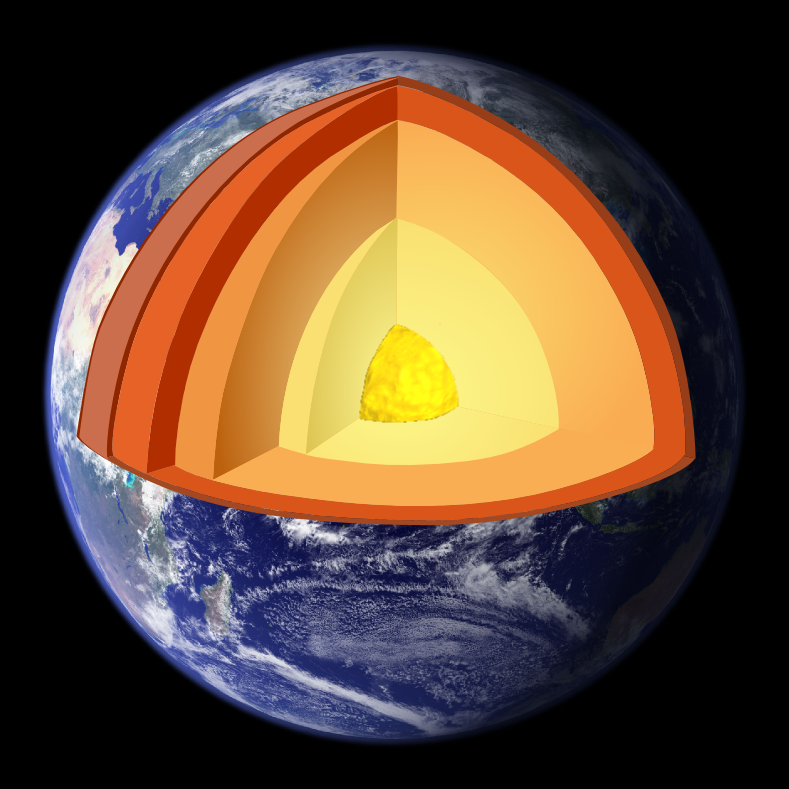
Seismology (/saɪzˈmɒlədʒi, saɪs-/; from Ancient Greek σεισμός (seismós) meaning "earthquake" and -λογία (-logía) meaning "study of") is the scientific study of earthquakes (or generally, quakes) and the generation and propagation of elastic waves through planetary bodies. It also includes studies of the environmental effects of earthquakes such as tsunamis; other seismic sources such as volcanoes, plate tectonics, glaciers, rivers, oceanic microseisms, and the atmosphere; and artificial processes such as explosions.
Paleoseismology is a related field that uses geology to infer information regarding past earthquakes. A recording of Earth's motion as a function of time, created by a seismograph is called a seismogram. A seismologist is a scientist who works in basic or applied seismology.
History
[edit]Scholarly interest in earthquakes can be traced back to antiquity. Early speculations on the natural causes of earthquakes were included in the writings of Thales of Miletus (c. 585 BCE), Anaximenes of Miletus (c. 550 BCE), Aristotle (c. 340 BCE), and Zhang Heng (132 CE).
In 132 CE, Zhang Heng of China's Han dynasty designed the first known seismoscope.[1][2][3]
In the 17th century, Athanasius Kircher argued that earthquakes were caused by the movement of fire within a system of channels inside the Earth. Martin Lister (1638–1712) and Nicolas Lemery (1645–1715) proposed that earthquakes were caused by chemical explosions within the Earth.[4]
The Lisbon earthquake of 1755, coinciding with the general flowering of science in Europe, set in motion intensified scientific attempts to understand the behaviour and causation of earthquakes. The earliest responses include work by John Bevis (1757) and John Michell (1761). Michell determined that earthquakes originate within the Earth and were waves of movement caused by "shifting masses of rock miles below the surface".[5]
In response to a series of earthquakes near Comrie in Scotland in 1839, a committee was formed in the United Kingdom in order to produce better detection methods for earthquakes. The outcome of this was the production of one of the first modern seismometers by James David Forbes, first presented in a report by David Milne-Home in 1842.[6] This seismometer was an inverted pendulum, which recorded the measurements of seismic activity through the use of a pencil placed on paper above the pendulum. The designs provided did not prove effective, according to Milne's reports.[6]
From 1857, Robert Mallet laid the foundation of modern instrumental seismology and carried out seismological experiments using explosives. He is also responsible for coining the word "seismology."[7] He is widely considered to be the "Father of Seismology".
In 1889 Ernst von Rebeur-Paschwitz recorded the first teleseismic earthquake signal (an earthquake in Japan recorded at Pottsdam Germany).[8]
In 1897, Emil Wiechert's theoretical calculations led him to conclude that the Earth's interior consists of a mantle of silicates, surrounding a core of iron.[9]
In 1906 Richard Dixon Oldham identified the separate arrival of P waves, S waves and surface waves on seismograms and found the first clear evidence that the Earth has a central core.[10]
In 1909, Andrija Mohorovičić, one of the founders of modern seismology,[11][12][13] discovered and defined the Mohorovičić discontinuity.[14] Usually referred to as the "Moho discontinuity" or the "Moho," it is the boundary between the Earth's crust and the mantle. It is defined by the distinct change in velocity of seismological waves as they pass through changing densities of rock.[15]
In 1910, after studying the April 1906 San Francisco earthquake, Harry Fielding Reid put forward the "elastic rebound theory" which remains the foundation for modern tectonic studies. The development of this theory depended on the considerable progress of earlier independent streams of work on the behavior of elastic materials and in mathematics.[16]
An early scientific study of aftershocks from a destructive earthquake came after the January 1920 Xalapa earthquake. An 80 kg (180 lb) Wiechert seismograph was brought to the Mexican city of Xalapa by rail after the earthquake. The instrument was deployed to record its aftershocks. Data from the seismograph would eventually determine that the mainshock was produced along a shallow crustal fault.[17]
In 1926, Harold Jeffreys was the first to claim, based on his study of earthquake waves, that below the mantle, the core of the Earth is liquid.[18]
In 1937, Inge Lehmann determined that within Earth's liquid outer core there is a solid inner core.[19]
In 1950, Michael S. Longuet-Higgins elucidated the ocean processes responsible for the global background seismic microseism.[20]
By the 1960s, Earth science had developed to the point where a comprehensive theory of the causation of seismic events and geodetic motions had come together in the now well-established theory of plate tectonics.[21]
Types of seismic wave
[edit]
Seismic waves are elastic waves that propagate in solid or fluid materials. They can be divided into body waves that travel through the interior of the materials; surface waves that travel along surfaces or interfaces between materials; and normal modes, a form of standing wave.
Body waves
[edit]There are two types of body waves, pressure waves or primary waves (P waves) and shear or secondary waves (S waves). P waves are longitudinal waves associated with compression and expansion, and involve particle motion parallel to the direction of wave propagation. P waves are always the first waves to appear on a seismogram as they are the waves that travel fastest through solids. S waves are transverse waves associated with shear, and involve particle motion perpendicular to the direction of wave propagation. S waves travel more slowly than P waves so they appear later than P waves on a seismogram. Because of their low shear strength, fluids cannot support transverse elastic waves, so S waves travel only in solids.[22]
Surface waves
[edit]Surface waves are the result of P and S waves interacting with the surface of the Earth. These waves are dispersive, meaning that different frequencies have different velocities. The two main surface wave types are Rayleigh waves, which have both compressional and shear motions, and Love waves, which are purely shear. Rayleigh waves result from the interaction of P waves and vertically polarized S waves with the surface and can exist in any solid medium. Love waves are formed by horizontally polarized S waves interacting with the surface, and can only exist if there is a change in the elastic properties with depth in a solid medium, which is always the case in seismological applications. Surface waves travel more slowly than P waves and S waves because they are the result of these waves traveling along indirect paths to interact with Earth's surface. Because they travel along the surface of the Earth, their energy decays less rapidly than body waves (1/distance2 vs. 1/distance3), and thus the shaking caused by surface waves is generally stronger than that of body waves, and the primary surface waves are often thus the largest signals on earthquake seismograms. Surface waves are strongly excited when their source is close to the surface, as in a shallow earthquake or a near-surface explosion, and are much weaker for deep earthquake sources.[22]
Normal modes
[edit]Both body and surface waves are traveling waves; however, large earthquakes can also make the entire Earth "ring" like a resonant bell. This ringing is a mixture of normal modes with discrete frequencies and periods of approximately an hour or shorter. Normal-mode motion caused by a very large earthquake can be observed for up to a month after the event.[22] The first observations of normal modes were made in the 1960s as the advent of higher-fidelity instruments coincided with two of the largest earthquakes of the 20th century, the 1960 Valdivia earthquake and the 1964 Alaska earthquake. Since then, the normal modes of the Earth have given us some of the strongest constraints on the deep structure of the Earth.
Earthquakes
[edit]One of the first attempts at the scientific study of earthquakes followed the 1755 Lisbon earthquake. Other earthquakes that spurred major advancements in the science of seismology include the 1857 Basilicata earthquake, the 1906 San Francisco earthquake, the 1964 Alaska earthquake, the 2004 Sumatra-Andaman earthquake, and the 2011 Great East Japan earthquake.
Controlled seismic sources
[edit]Seismic waves produced by explosions or vibrating controlled sources are one of the primary methods of underground exploration in geophysics (in addition to many different electromagnetic methods such as induced polarization and magnetotellurics). Controlled-source seismology has been used to map salt domes, anticlines and other geologic traps in petroleum-bearing rocks, faults, rock types, and long-buried giant meteor craters. For example, the Chicxulub Crater, which was caused by an impact that has been implicated in the extinction of the dinosaurs, was localized to Central America by analyzing ejecta in the Cretaceous–Paleogene boundary, and then physically proven to exist using seismic maps from oil exploration.[23]
Detection of seismic waves
[edit]Seismometers are sensors that detect and record the motion of the Earth arising from elastic waves. Seismometers may be deployed at the Earth's surface, in shallow vaults, in boreholes, or underwater. A complete instrument package that records seismic signals is called a seismograph. Networks of seismographs continuously record ground motions around the world to facilitate the monitoring and analysis of global earthquakes and other sources of seismic activity. Rapid location of earthquakes makes tsunami warnings possible because seismic waves travel considerably faster than tsunami waves.
Seismometers also record signals from non-earthquake sources ranging from explosions (nuclear and chemical), to local noise from wind[24] or anthropogenic activities, to incessant signals generated at the ocean floor and coasts induced by ocean waves (the global microseism), to cryospheric events associated with large icebergs and glaciers. Above-ocean meteor strikes with energies as high as 4.2 × 10¹³ J (equivalent to that released by an explosion of ten kilotons of TNT) have been recorded by seismographs, as have a number of industrial accidents and terrorist bombs and events (a field of study referred to as forensic seismology). A major long-term motivation for the global seismographic monitoring has been for the detection and study of nuclear testing.
Mapping Earth's interior
[edit]
Because seismic waves commonly propagate efficiently as they interact with the internal structure of the Earth, they provide high-resolution noninvasive methods for studying the planet's interior. One of the earliest important discoveries (suggested by Richard Dixon Oldham in 1906 and definitively shown by Harold Jeffreys in 1926) was that the outer core of the earth is liquid. Since S waves do not pass through liquids, the liquid core causes a "shadow" on the side of the planet opposite the earthquake where no direct S waves are observed. In addition, P waves travel much slower through the outer core than the mantle.
Processing readings from many seismometers using seismic tomography, seismologists have mapped the mantle of the earth to a resolution of several hundred kilometers. This has enabled scientists to identify convection cells and other large-scale features such as the large low-shear-velocity provinces near the core–mantle boundary.[25]
Seismology and society
[edit]Earthquake prediction
[edit]Forecasting a probable timing, location, magnitude and other important features of a forthcoming seismic event is called earthquake prediction. Various attempts have been made by seismologists and others to create effective systems for precise earthquake predictions, including the VAN method. Most seismologists do not believe that a system to provide timely warnings for individual earthquakes has yet been developed, and many believe that such a system would be unlikely to give useful warning of impending seismic events. However, more general forecasts routinely predict seismic hazard. Such forecasts estimate the probability of an earthquake of a particular size affecting a particular location within a particular time-span, and they are routinely used in earthquake engineering.
Public controversy over earthquake prediction erupted after Italian authorities indicted six seismologists and one government official for manslaughter in connection with a magnitude 6.3 earthquake in L'Aquila, Italy on April 5, 2009.[26] A report in Nature stated that the indictment was widely seen in Italy and abroad as being for failing to predict the earthquake and drew condemnation from the American Association for the Advancement of Science and the American Geophysical Union.[26] However, the magazine also indicated that the population of Aquila do not consider the failure to predict the earthquake to be the reason for the indictment, but rather the alleged failure of the scientists to evaluate and communicate risk.[26] The indictment claims that, at a special meeting in L'Aquila the week before the earthquake occurred, scientists and officials were more interested in pacifying the population than providing adequate information about earthquake risk and preparedness.[26]
In locations where a historical record exists it may be used to estimate the timing, location and magnitude of future seismic events. There are several interpretative factors to consider. The epicentres or foci and magnitudes of historical earthquakes are subject to interpretation meaning it is possible that 5–6 Mw earthquakes described in the historical record could be larger events occurring elsewhere that were felt moderately in the populated areas that produced written records. Documentation in the historic period may be sparse or incomplete, and not give a full picture of the geographic scope of an earthquake, or the historical record may only have earthquake records spanning a few centuries, a very short time frame in a seismic cycle.[27][28]
Engineering seismology
[edit]Engineering seismology is the study and application of seismology for engineering purposes.[29] It generally applied to the branch of seismology that deals with the assessment of the seismic hazard of a site or region for the purposes of earthquake engineering. It is, therefore, a link between earth science and civil engineering.[30] There are two principal components of engineering seismology. Firstly, studying earthquake history (e.g. historical[30] and instrumental catalogs[31] of seismicity) and tectonics[32] to assess the earthquakes that could occur in a region and their characteristics and frequency of occurrence. Secondly, studying strong ground motions generated by earthquakes to assess the expected shaking from future earthquakes with similar characteristics. These strong ground motions could either be observations from accelerometers or seismometers or those simulated by computers using various techniques,[33] which are then often used to develop ground-motion prediction equations[34] (or ground-motion models)[1].
Tools
[edit]Seismological instruments can generate large amounts of data. Systems for processing such data include:
- CUSP (Caltech-USGS Seismic Processing)[35]
- RadExPro seismic software
- SeisComP3[36]
List of seismologists
[edit]- Aki, Keiiti
- Ambraseys, Nicholas
- Anderson, Don L.
- Bolt, Bruce
- Beroza, Gregory
- Claerbout, Jon
- Dziewonski, Adam Marian
- Ewing, Maurice
- Galitzine, Boris Borisovich
- Gamburtsev, Grigory A.
- Gutenberg, Beno
- Hough, Susan
- Jeffreys, Harold
- Jones, Lucy
- Kanamori, Hiroo
- Keilis-Borok, Vladimir
- Knopoff, Leon
- Lehmann, Inge
- Macelwane, James
- Mallet, Robert
- Mercalli, Giuseppe
- Milne, John
- Mohorovičić, Andrija
- Oldham, Richard Dixon
- Omori, Fusakichi
- Sebastião de Melo, Marquis of Pombal
- Press, Frank
- Rautian, Tatyana G.
- Richards, Paul G.
- Richter, Charles Francis
- Sekiya, Seikei
- Sieh, Kerry
- Paul G. Silver
- Stein, Ross
- Tucker, Brian
- Vidale, John
- Wen, Lianxing
- Winthrop, John
- Zhang Heng
See also
[edit]- Asteroseismology – Study of oscillations in stars (starquakes)
- Cryoseism – Non-tectonic seismic event
- Earthquake swarm – Series of localized seismic events within a short time period
- Engineering geology – Application of geology to engineering practice
- Epicentral distance
- Harmonic tremor – Sustained ground vibration associated with underground movement of magma or volcanic gas
- Helioseismology – Study of the structure and dynamics of the Sun through its oscillation
- IRIS Consortium – Former research group using seismographic data
- Isoseismal map – Type of map used in seismology
- Linear seismic inversion – Interpretation of seismic data using linear model
- Lunar seismology – Study of ground motions of the Moon
- Marsquake – Seismic event occurring on Mars
- Quake (natural phenomenon) – Surface shaking on interstellar bodies in general
- Seismic interferometry
- Seismic loading
- Seismic migration – Measurement process
- Seismic noise – Generic name for a relatively persistent vibration of the ground
- Seismic performance analysis – Study of the response of buildings and structures to earthquakes
- Seismic velocity structure – Seismic wave velocity variation
- Seismite – Sediment/structure shaken seismically
- Seismo-electromagnetics – Electro-magnetic phenomena
- Seismotectonics
- Stabilized inverse Q filtering – Data processing technology
Notes
[edit]- ^ Needham, Joseph (1959). Science and Civilization in China, Volume 3: Mathematics and the Sciences of the Heavens and the Earth. Cambridge: Cambridge University Press. pp. 626–635. Bibcode:1959scc3.book.....N.
- ^ Dewey, James; Byerly, Perry (February 1969). "The early history of seismometry (to 1900)". Bulletin of the Seismological Society of America. 59 (1): 183–227.
- ^ Agnew, Duncan Carr (2002). "History of seismology". International Handbook of Earthquake and Engineering Seismology. International Geophysics. 81A: 3–11. Bibcode:2002InGeo..81....3A. doi:10.1016/S0074-6142(02)80203-0. ISBN 9780124406520.
- ^ Udías, Agustín; Arroyo, Alfonso López (2008). "The Lisbon earthquake of 1755 in Spanish contemporary authors". In Mendes-Victor, Luiz A.; Oliveira, Carlos Sousa; Azevedo, João; Ribeiro, Antonio (eds.). The 1755 Lisbon earthquake: revisited. Springer. p. 14. ISBN 9781402086090.
- ^ Member of the Royal Academy of Berlin (2012). The History and Philosophy of Earthquakes Accompanied by John Michell's 'conjectures Concerning the Cause, and Observations upon the Ph'nomena of Earthquakes'. Cambridge Univ Pr. ISBN 9781108059909.
- ^ a b Oldroyd, David (2007). "The Study of Earthquakes in the Hundred Years Following Lisbon Earthquake of 1755". Researchgate. Earth sciences history: journal of the History of the Earth Sciences Society. Retrieved 4 October 2022.
- ^ Society, The Royal (2005-01-22). "Robert Mallet and the 'Great Neapolitan earthquake' of 1857". Notes and Records. 59 (1): 45–64. doi:10.1098/rsnr.2004.0076. ISSN 0035-9149. S2CID 71003016.
- ^ "Historical Seismograms from the Potsdam Station" (PDF). Academy of Sciences of German Democratic Republic, Central Institute for the Physics of the Earth. 1989. Retrieved April 7, 2020.
- ^ Barckhausen, Udo; Rudloff, Alexander (14 February 2012). "Earthquake on a stamp: Emil Wiechert honored". Eos, Transactions American Geophysical Union. 93 (7): 67. Bibcode:2012EOSTr..93...67B. doi:10.1029/2012eo070002.
- ^ "Oldham, Richard Dixon". Complete Dictionary of Scientific Biography. Vol. 10. Charles Scribner's Sons. 2008. p. 203.
- ^ "Andrya (Andrija) Mohorovicic". Penn State. Archived from the original on 26 June 2013. Retrieved 30 January 2021.
- ^ "Mohorovičić, Andrija". Encyclopedia.com. Archived from the original on 1 February 2021. Retrieved 30 January 2021.
- ^ "Andrija Mohorovičić (1857–1936) – On the occasion of the 150th anniversary of his birth". Seismological Society of America. Archived from the original on 1 February 2021. Retrieved 30 January 2021.
- ^ Andrew McLeish (1992). Geological science (2nd ed.). Thomas Nelson & Sons. p. 122. ISBN 978-0-17-448221-5.
- ^ Rudnick, R. L.; Gao, S. (2003-01-01), Holland, Heinrich D.; Turekian, Karl K. (eds.), "3.01 – Composition of the Continental Crust", Treatise on Geochemistry, 3, Pergamon: 659, Bibcode:2003TrGeo...3....1R, doi:10.1016/b0-08-043751-6/03016-4, ISBN 978-0-08-043751-4, retrieved 2019-11-21
- ^ "Reid's Elastic Rebound Theory". 1906 Earthquake. United States Geological Survey. Retrieved 6 April 2018.
- ^ Suárez, G.; Novelo-Casanova, D. A. (2018). "A Pioneering Aftershock Study of the Destructive 4 January 1920 Jalapa, Mexico, Earthquake". Seismological Research Letters. 89 (5): 1894–1899. Bibcode:2018SeiRL..89.1894S. doi:10.1785/0220180150. S2CID 134449441.
- ^ Jeffreys, Harold (1926-06-01). "On the Amplitudes of Bodily Seismic Waues". Geophysical Journal International. 1: 334–348. Bibcode:1926GeoJ....1..334J. doi:10.1111/j.1365-246X.1926.tb05381.x. ISSN 1365-246X.
- ^ Hjortenberg, Eric (December 2009). "Inge Lehmann's work materials and seismological epistolary archive". Annals of Geophysics. 52 (6). doi:10.4401/ag-4625.
- ^ Longuet-Higgins, M. S. (1950), "A theory of the origin of microseisms", Philosophical Transactions of the Royal Society A, 243 (857): 1–35, Bibcode:1950RSPTA.243....1L, doi:10.1098/rsta.1950.0012, S2CID 31828394
- ^ "History of plate tectonics". scecinfo.usc.edu. Retrieved 2024-02-20.
- ^ a b c Gubbins 1990
- ^ Schulte et al. 2010
- ^ Naderyan, Vahid; Hickey, Craig J.; Raspet, Richard (2016). "Wind-induced ground motion". Journal of Geophysical Research: Solid Earth. 121 (2): 917–930. Bibcode:2016JGRB..121..917N. doi:10.1002/2015JB012478.
- ^ Wen & Helmberger 1998
- ^ a b c d Hall 2011
- ^ Historical Seismology: Interdisciplinary Studies of Past and Recent Earthquakes(2008) Springer Netherlands
- ^ Thakur, Prithvi; Huang, Yihe (2021). "Influence of Fault Zone Maturity on Fully Dynamic Earthquake Cycles". Geophysical Research Letters. 48 (17). Bibcode:2021GeoRL..4894679T. doi:10.1029/2021GL094679. hdl:2027.42/170290.
- ^ Plimer, Richard C. SelleyL. Robin M. CocksIan R., ed. (2005-01-01). "Editors". Encyclopaedia of Geology. Oxford: Elsevier. pp. 499–515. doi:10.1016/b0-12-369396-9/90020-0. ISBN 978-0-12-369396-9.
- ^ a b Ambraseys, N. N. (1988-12-01). "Engineering seismology: Part I". Earthquake Engineering & Structural Dynamics. 17 (1): 1–50. Bibcode:1988EESD...17....1A. doi:10.1002/eqe.4290170101. ISSN 1096-9845.
- ^ Wiemer, Stefan (2001-05-01). "A Software Package to Analyze Seismicity: ZMAP". Seismological Research Letters. 72 (3): 373–382. Bibcode:2001SeiRL..72..373W. doi:10.1785/gssrl.72.3.373. ISSN 0895-0695.
- ^ Bird, Peter; Liu, Zhen (2007-01-01). "Seismic Hazard Inferred from Tectonics: California". Seismological Research Letters. 78 (1): 37–48. Bibcode:2007SeiRL..78...37B. doi:10.1785/gssrl.78.1.37. ISSN 0895-0695.
- ^ Douglas, John; Aochi, Hideo (2008-10-10). "A Survey of Techniques for Predicting Earthquake Ground Motions for Engineering Purposes" (PDF). Surveys in Geophysics. 29 (3): 187–220. Bibcode:2008SGeo...29..187D. doi:10.1007/s10712-008-9046-y. ISSN 0169-3298. S2CID 53066367.
- ^ Douglas, John; Edwards, Benjamin (2016-09-01). "Recent and future developments in earthquake ground motion estimation" (PDF). Earth-Science Reviews. 160: 203–219. Bibcode:2016ESRv..160..203D. doi:10.1016/j.earscirev.2016.07.005.
- ^
Lee, W. H. K.; S. W. Stewart (1989). "Large-Scale Processing and Analysis of Digital Waveform Data from the USGS Central California Microearthquake Network". Observatory seismology: an anniversary symposium on the occasion of the centennial of the University of California at Berkeley seismographic stations. University of California Press. p. 86. ISBN 9780520065826. Retrieved 2011-10-12.
The CUSP (Caltech-USGS Seismic Processing) System consists of on-line real-time earthquake waveform data acquisition routines, coupled with an off-line set of data reduction, timing, and archiving processes. It is a complete system for processing local earthquake data ...
- ^ Akkar, Sinan; Polat, Gülkan; van Eck, Torild, eds. (2010). Earthquake Data in Engineering Seismology: Predictive Models, Data Management and Networks. Geotechnical, Geological and Earthquake Engineering. Vol. 14. Springer. p. 194. ISBN 978-94-007-0151-9. Retrieved 2011-10-19.
References
[edit]- Allaby, Ailsa; Allaby, Michael, eds. (2003). Oxford Dictionary of Earth Sciences (2nd ed.). Oxford University Press.
- Ben-Menahem, Ari (1995), "A Concise History of Mainstream Seismology: Origins, Legacy, and Perspectives" (PDF), Bulletin of the Seismological Society of America, 85 (4): 1202–1225
- Bath, M. (1979). Introduction to Seismology (2nd rev. ed.). Basel: Birkhäuser Basel. ISBN 9783034852838.
- Davison, Charles (2014). The founders of seismology. Cambridge University Press. ISBN 9781107691490.
- Ewing, W. M.; Jardetzky, W. S.; Press, F. (1957). Elastic Waves in Layered Media. McGraw-Hill Book Company.
- Gubbins, David (1990). Seismology and Plate Tectonics. Cambridge University Press. ISBN 978-0-521-37141-4.
- Hall, Stephen S. (2011). "Scientists on trial: At fault?". Nature. 477 (7364): 264–269. Bibcode:2011Natur.477..264H. doi:10.1038/477264a. PMID 21921895. S2CID 205067216.
- Kanamori, Hiroo (2003). Earthquake prediction: An overview (PDF). International Handbook of Earthquake and Engineering Seismology. Vol. 81B. International Association of Seismology & Physics of the Earth's Interior. pp. 1205–1216. Archived from the original (PDF) on 2013-10-24.
- Lay, Thorne, ed. (2009). Seismological Grand Challenges in Understanding Earth's Dynamic Systems (PDF). Report to the National Science Foundation, IRIS consortium.
- Schulte, Peter; Laia Alegret; Ignacio Arenillas; José A. Arz; Penny J. Barton; Paul R. Bown; Timothy J. Bralower; Gail L. Christeson; Philippe Claeys; Charles S. Cockell; Gareth S. Collins; Alexander Deutsch; Tamara J. Goldin; Kazuhisa Goto; José M. Grajales-Nishimura; Richard A. F. Grieve; Sean P. S. Gulick; Kirk R. Johnson; Wolfgang Kiessling; Christian Koeberl; David A. Kring; Kenneth G. MacLeod; Takafumi Matsui; Jay Melosh; Alessandro Montanari; Joanna V. Morgan; Clive R. Neal; Douglas J. Nichols; Richard D. Norris; Elisabetta Pierazzo; Greg Ravizza; Mario Rebolledo-Vieyra; Wolf Uwe Reimold; Eric Robin; Tobias Salge; Robert P. Speijer; Arthur R. Sweet; Jaime Urrutia-Fucugauchi; Vivi Vajda; Michael T. Whalen; Pi S. Willumsen (5 March 2010). "The Chicxulub Asteroid Impact and Mass Extinction at the Cretaceous-Paleogene Boundary". Science. 327 (5970): 1214–1218. Bibcode:2010Sci...327.1214S. doi:10.1126/science.1177265. ISSN 1095-9203. PMID 20203042. S2CID 2659741. Retrieved 5 March 2010.
- Shearer, Peter M. (2009). Introduction to Seismology (2nd ed.). Cambridge University Press. ISBN 978-0-521-70842-5.
- Stein, Seth; Wysession, Michael (2002). An Introduction to Seismology, Earthquakes and Earth Structure. Wiley-Blackwell. ISBN 978-0-86542-078-6.
- Wen, Lianxing; Helmberger, Donald V. (1998). "Ultra-Low Velocity Zones Near the Core-Mantle Boundary from Broadband PKP Precursors" (PDF). Science. 279 (5357): 1701–1703. Bibcode:1998Sci...279.1701W. doi:10.1126/science.279.5357.1701. PMID 9497284.
External links
[edit]Seismology
View on GrokipediaFundamentals of Seismology
Definition and Core Principles
Seismology is the scientific discipline dedicated to the study of earthquakes and the propagation of elastic waves through the Earth and other planetary bodies, utilizing data from these waves to infer internal structures and material properties.[9] These elastic waves, known as seismic waves, are generated primarily by natural events such as tectonic earthquakes or volcanic activity, as well as artificial sources like explosions, and are recorded using seismographs to produce seismograms—traces of ground motion over time.[10] The field relies on empirical observations of wave arrivals and characteristics to model the Earth's subsurface, revealing discontinuities such as the Mohorovičić discontinuity separating the crust from the mantle, first identified in 1909 through travel-time analysis of waves from the 1909 Kulpa Valley earthquake in Croatia.[11] At its foundation, seismology operates on principles of elastodynamics, where seismic waves satisfy the elastic wave equation derived from Hooke's law and Newton's second law, describing particle displacements in a continuum medium with shear modulus μ and compressional modulus λ + 2μ.[12] Body waves include compressional P-waves, which propagate via alternating compression and dilation at velocities up to 13.5 km/s in the upper mantle, and shear S-waves, which involve transverse motion at about 60% of P-wave speeds and cannot traverse fluids like the outer core.[13] Wave speeds vary with depth due to gradients in density ρ and elastic moduli, governed by Poisson's ratio σ = (λ)/(2(λ + μ)), typically around 0.25 for crustal rocks, enabling refraction and reflection at interfaces per Snell's law.[11] Attenuation, the loss of wave amplitude through anelastic processes like viscoelastic damping, follows an exponential decay e^{-α r} where α is the attenuation coefficient and r distance, quantified by quality factor Q = 2π (energy stored / energy dissipated per cycle), with higher Q in the mantle (around 100-1000) indicating lower dissipation than in the crust.[12] Surface waves, such as Rayleigh and Love waves, dominate long-period ground motion and exhibit dispersive propagation, with phase velocities depending on frequency due to waveguide effects in layered media.[14] These principles, applied to global networks of over 10,000 broadband seismometers as of 2023, have delineated the Earth's core-mantle boundary at approximately 2890 km depth, where P-waves slow abruptly and S-waves vanish, confirming a liquid outer core.[14]Types of Seismic Waves
Seismic waves produced by earthquakes are divided into body waves, which travel through the Earth's interior, and surface waves, which propagate along or near the surface. Body waves include primary (P) waves and secondary (S) waves, while surface waves comprise Love waves and Rayleigh waves. These waves differ in particle motion, speed, and ability to traverse materials, providing insights into Earth's structure based on their arrival times at seismometers.[15][16] P waves, also known as compressional or longitudinal waves, are the fastest seismic waves, traveling at velocities of approximately 5-8 km/s in the crust. They cause particles in the medium to oscillate parallel to the direction of wave propagation, akin to sound waves, and can propagate through solids, liquids, and gases. This property allowed P waves to reveal the existence of Earth's liquid outer core, as they refract at the core-mantle boundary. P waves arrive first at recording stations, enabling initial earthquake detection.[17][18] S waves, or shear waves, exhibit transverse motion where particles move perpendicular to the wave's direction, typically at speeds of 3-4.5 km/s in the crust, about 60% of P wave velocity. Unlike P waves, S waves cannot travel through liquids, as shear stress does not transmit in fluids, confirming the outer core's liquidity when S waves are absent beyond certain distances. They produce stronger ground shaking than P waves due to their slower speed and larger amplitudes in solids.[17][18] Love waves, named after Augustus Edward Hough Love who mathematically described them in 1911, are horizontally polarized surface waves that cause particle motion parallel to the surface and perpendicular to propagation, resembling S wave behavior but confined near the surface. They travel slightly faster than Rayleigh waves, at around 2-4 km/s depending on frequency and depth, and are dispersive, with velocity varying by wavelength. Love waves contribute significantly to seismic damage through horizontal shearing.[19][20] Rayleigh waves, theorized by Lord Rayleigh in 1885, produce elliptical, retrograde particle motion in a vertical plane aligned with propagation, rolling like ocean waves along the surface. Their speed is slightly less than S waves, approximately 90% of S wave velocity, and they too are dispersive. Rayleigh waves typically cause the most extensive ground displacement and are responsible for much of the destructive shaking in earthquakes, as their energy decays slowly with depth.[19][20]Propagation and Attenuation
Seismic waves propagate through Earth's interior primarily as body waves, which include compressional primary (P) waves and shear secondary (S) waves, traveling through the full volume of the planet. P-waves consist of alternating compressions and dilations parallel to the direction of propagation, enabling them to traverse both solids and fluids, while S-waves involve particle motion perpendicular to propagation and are restricted to solids.[21][22] Velocities of P-waves increase from approximately 6 km/s in the crust to 13 km/s in the lower mantle due to increasing pressure and density with depth, causing wave paths to refract and curve according to Snell's law at layer boundaries.[23] S-wave velocities follow similar gradients, typically about 60% of P-wave speeds, such as 3.5 km/s in the crust and 7 km/s in the mantle.[22] Surface waves, including Love and Rayleigh types, propagate along the Earth's surface or interfaces, generally slower than body waves with velocities around 3-4.5 km/s, and are confined to shallower depths, leading to greater amplitudes and prolonged ground motion.[21] Love waves feature horizontally transverse particle motion, while Rayleigh waves produce elliptical retrograde orbits in the vertical plane.[22] Wave propagation is governed by the elastic wave equation, with paths influenced by spherical geometry and radial velocity variations, resulting in shadow zones for direct P and S arrivals beyond 103-105 degrees epicentral distance due to core refraction.[9][23] Attenuation of seismic waves occurs through multiple mechanisms, reducing amplitude with distance and frequency. Geometric spreading causes amplitude decay proportional to inverse distance for body waves (1/r) due to energy distribution over expanding wavefronts, and inversely proportional to the square root of distance for surface waves (1/√r).[24][25] Inelastic absorption dissipates energy as heat via internal friction in the medium, quantified by the quality factor Q, where higher Q indicates less attenuation; typical crustal Q values range from 100-1000, increasing with depth.[24][26] Scattering redirects energy into diffuse coda waves due to heterogeneities, dominating high-frequency attenuation in regions like Southern California, often exceeding intrinsic absorption effects.[27][28] Overall attenuation combines these effects, with frequency-dependent Q models describing exponential decay, e^{ -π f t / Q }, where f is frequency and t is travel time.[29][25]Historical Development
Ancient and Early Modern Observations
Ancient Greek philosophers provided some of the earliest systematic observations and theories of earthquakes, attributing them to natural subterranean processes rather than solely divine intervention. Thales of Miletus (c. 640–546 BC) proposed that the Earth floats on water, with earthquakes resulting from oceanic movements.[30] Anaximenes (c. 585–524 BC) suggested that extreme moisture or dryness caused the Earth to crack internally, leading to shaking.[30] Aristotle (384–322 BC), in his Meteorology (c. 350 BC), advanced a comprehensive theory based on collected reports from regions like Greece, Sicily, and the Hellespont: earthquakes arise from dry exhalations (vapors) generated by solar heat interacting with subterranean moisture, forming winds trapped in caverns that exert pressure and shake the Earth upon release or confinement.[31][30] He noted empirical patterns, such as greater frequency in porous, cavernous terrains, during calm weather (especially night or noon), spring and autumn seasons, and associations with phenomena like wells running dry or unusual animal behavior beforehand, though these lacked causal mechanisms beyond wind dynamics.[31] Roman writers built on Greek ideas while documenting specific events. Seneca the Younger (c. 4 BC–AD 65), in Naturales Quaestiones, referenced earthquakes in Campania and Asia Minor, endorsing wind-based causes similar to Aristotle but emphasizing rhetorical descriptions of rumbling sounds and prolonged shocks lasting up to days.[30] In parallel, ancient China maintained detailed historical records of seismic events dating back to the Shang Dynasty (c. 1600–1046 BC), with systematic catalogs emerging by the Han Dynasty (206 BC–AD 220), including notations of date, location, damage, and portents like animal distress.[32] Zhang Heng (AD 78–139), a Han polymath serving as court astrologer, invented a seismoscope in AD 132: a bronze vessel with eight dragon heads positioned by compass directions, each holding a ball above a toad mouth; seismic waves displaced an internal pendulum, causing a ball to drop from the corresponding dragon, indicating the quake's origin direction without measuring intensity or time.[33] Historical accounts claim it detected a magnitude ~5 earthquake in Longxi (over 400 km distant) before local tremors arrived, alerting the court; however, modern replicas achieve only limited sensitivity (detecting nearby quakes), failing to replicate the reported range, raising questions about potential embellishment in records or unrecovered design details.[34] Early modern European observations, from the 17th to 18th centuries, increasingly emphasized eyewitness testimonies over mythology, facilitated by networks like the Royal Society, which solicited accounts of tremors in England (e.g., 1692 Jamaica quake felt in Europe) and Italy.[35] These described wave-like ground motion, underground noises, and propagation speeds inferred from timed reports across distances. The 1755 Lisbon earthquake marked a pivotal observational benchmark: on November 1, a sequence of shocks (initial lasting 6–7 minutes) struck at ~9:40 AM, with estimated magnitude 8.5–9.0, liquefying soil, igniting fires, and triggering a 6–20 m tsunami that propagated to Morocco and beyond, causing ~60,000 deaths.[36][35] Contemporary letters and surveys documented isoseismal patterns, foreshocks, and aftershocks persisting months, with felt reports extending to Finland and the West Indies, enabling early estimates of epicentral location off Portugal's coast—though interpretations remained tied to flawed models like subterranean explosions rather than tectonic faulting.[35][36]Establishment of Seismology as a Science
The systematic establishment of seismology as a scientific discipline emerged in the late 19th century, driven by the invention of recording seismographs that shifted studies from qualitative observations to quantitative measurements of seismic waves. Prior to this, earthquake investigations were largely descriptive, influenced by events like the 1755 Lisbon earthquake, which prompted early modern analyses but lacked instrumental precision.[37][38] Pioneering efforts included the installation of one of the earliest seismographs by Jesuit missionaries in Manila in 1868, marking the beginning of instrumental monitoring in a seismically active region.[39] In Italy, Filippo Cecchi developed a low-sensitivity recording seismograph around 1875, capable of documenting local tremors.[40] These devices laid groundwork, but broader adoption accelerated in the 1880s with innovations by Scottish physicist James Alfred Ewing, engineer Thomas Gray, and British geologist John Milne, who collaboratively invented the horizontal pendulum seismograph in 1880 while in Japan. This instrument improved sensitivity and enabled detection of distant earthquakes, facilitating global data collection.[41][42] The 1883 eruption of Krakatoa volcano provided a critical test, as its seismic signals were recorded worldwide by emerging networks, demonstrating the potential for studying wave propagation across Earth.[43] This event, combined with the establishment of seismological observatories—such as those in Japan following Milne's work and in Europe—solidified seismology's scientific status by the 1890s. Standardized intensity scales, like the Rossi-Forel scale introduced around 1883, further supported empirical classification of shaking effects.[43] By the early 20th century, these advancements enabled the first global seismic recordings, such as the 1889 Potsdam event, confirming seismology's transition to a rigorous, data-driven field.[44]20th-Century Advances and Key Discoveries
The early 20th century saw foundational insights into Earth's crustal structure through analysis of seismic wave velocities. In 1909, following a magnitude approximately 6.0 earthquake in Croatia's Kulpa Valley on October 8, Andrija Mohorovičić observed an abrupt increase in P-wave velocity from about 6 km/s to 8 km/s at a depth of roughly 30 km beneath the epicenter, interpreting this as the boundary separating the crust from the denser mantle; this interface, termed the Mohorovičić discontinuity or Moho, represented the first seismic evidence of lateral heterogeneity in Earth's layers.[45][46] Advancements in understanding the deep interior followed from refined wave path modeling and global earthquake records. German-American seismologist Beno Gutenberg, building on observations of P-wave shadow zones—regions where direct P-waves from distant earthquakes failed to arrive—calculated the core-mantle boundary depth at 2,900 km in 1913 and proposed a liquid outer core to explain the absence of S-waves beyond this depth, as S-waves cannot propagate through liquids.[47] In 1936, Danish seismologist Inge Lehmann identified reflected P' waves in data from South American and New Zealand earthquakes, inferring a solid inner core boundary at about 5,100 km depth where waves transitioned from liquid to solid material, overturning prior assumptions of a fully liquid core; this discovery relied on meticulous reanalysis of faint seismic signals amid noise.[48][5] Instrumental innovations enabled quantitative earthquake assessment and broader data collection. In 1906, Russian physicist Boris Golitsyn invented the first effective electromagnetic seismograph, providing sensitive, broadband measurements that advanced quantitative seismic recording.[49] In 1935, Charles F. Richter, collaborating with Gutenberg at the California Institute of Technology, developed the local magnitude scale (ML), a logarithmic measure defined as ML = log10(A) + correction factors for distance and instrument response, where A is the maximum trace amplitude in millimeters on a Wood-Anderson seismograph; initially calibrated for southern California earthquakes with magnitudes up to about 7, it provided a standardized metric for comparing event sizes independent of subjective intensity reports.[50] Post-World War II, controlled-source seismology using explosions for crustal profiling advanced Moho mapping, revealing average continental crustal thicknesses of 30-50 km.[51] By mid-century, expanded networks transformed seismology into a global science underpinning tectonic theory. The Worldwide Standardized Seismograph Network (WWSSN), deployed in 1961 with over 120 uniform long- and short-period stations, enhanced detection of teleseisms and focal depths, yielding data that delineated linear earthquake belts along mid-ocean ridges and subduction zones—key evidence for rigid lithospheric plates moving at 1-10 cm/year, as formalized in plate tectonics by the late 1960s; seismic moment tensors from these records confirmed strike-slip, thrust, and normal faulting consistent with plate boundary mechanics.[52] These developments shifted seismology from descriptive recording to predictive modeling of Earth's dynamic interior.[53]Seismic Sources
Natural Tectonic Earthquakes
Natural tectonic earthquakes result from the sudden release of elastic strain energy accumulated in the Earth's crust due to the movement of tectonic plates. These plates, rigid segments of the lithosphere, shift at rates of a few centimeters per year, driven by convection in the mantle, but friction along their boundaries locks them in place, building stress until it overcomes resistance and causes brittle failure along faults.[54][55] This process accounts for the vast majority of seismic events, distinct from volcanic or induced seismicity, as it stems directly from lithospheric deformation rather than magma movement or human activity.[54] The elastic rebound theory, formulated by Harry Fielding Reid following the 1906 San Francisco earthquake, explains the mechanism: rocks on either side of a fault deform elastically under sustained stress, storing potential energy like a bent spring; upon rupture, they rebound to their original configuration, propagating seismic waves.[56] Faults are fractures where such slip occurs, classified by motion: strike-slip faults involve horizontal shearing, as along the San Andreas Fault; normal faults feature extension with one block dropping relative to the other; and thrust (reverse) faults involve compression, one block overriding another, common in subduction zones.[57] These styles correlate with plate boundary types—divergent, transform, and convergent—determining rupture characteristics and energy release.[58] Globally, tectonic earthquakes cluster along plate boundaries, forming narrow belts like the circum-Pacific Ring of Fire, where approximately 90% of events occur due to subduction and transform interactions.[59] Other zones include mid-ocean ridges and intraplate features like the New Madrid Seismic Zone, though less frequent. Depths typically range from shallow crustal levels (<70 km) to intermediate (70-300 km) in subduction settings, with energy release scaling logarithmically via the moment magnitude scale.[60] Annually, the planet experiences about 12,000 to 14,000 detectable earthquakes, predominantly tectonic, with magnitudes distributed as follows: roughly 1,300 above 5.0, 130 above 6.0, 15 above 7.0, and 1 above 8.0, though great events (M>8) vary interannually.[61][62] These statistics, derived from global networks, underscore the predictability of locations but variability in timing and size, informing hazard assessment through recurrence intervals and paleoseismic records.[61]Volcanic and Other Natural Sources
Volcanic seismicity arises from processes involving magma ascent, fluid migration, and pressure variations within volcanic systems, often serving as precursors to eruptions. These events are distinguished by their shallow focal depths, typically ranging from 1 to 10 kilometers, compared to the deeper origins of tectonic earthquakes. Seismic signals from volcanoes include discrete earthquakes and continuous tremors, driven by interactions between molten rock, hydrothermal fluids, and surrounding rock.[63][64] Volcano-tectonic (VT) earthquakes, one primary type, occur due to brittle shear failure along faults induced by stress perturbations from magma intrusion or edifice loading. They produce high-frequency P- and S-waves akin to tectonic events, with frequencies around 5-10 Hz, and can reach magnitudes up to 5 or higher.[65][66] Long-period (LP) earthquakes, by contrast, feature emergent onsets and dominant frequencies of 0.5-5 Hz, attributed to volumetric changes from fluid excitation or resonance in fluid-filled fractures and conduits.[66] Hybrid earthquakes combine VT and LP traits, while volcanic tremor manifests as prolonged, low-frequency (1-5 Hz) oscillations from sustained magma or gas flow.[66] These signals often cluster before eruptive activity, aiding monitoring; for instance, increased VT seismicity preceded the 1980 Mount St. Helens eruption, with a notable magnitude 5.5 VT event in 1981 marking one of the strongest recorded in the U.S. Cascades.[65] Beyond volcanism, other natural non-tectonic sources generate detectable seismic waves through mass wasting or extraterrestrial impacts. Large landslides, particularly in glaciated terrains, displace substantial volumes of material, producing seismic signals that can register as low-frequency events with magnitudes exceeding 4, distinguishable by their surface-wave dominance and lack of deep focal mechanisms. In the Puget Sound region, glacial deposits contribute to frequent landslides that yield microseismic signals monitored for hazard assessment.[67][68] Glacial earthquakes, concentrated in ice-covered areas like Greenland and Alaska, stem from abrupt sliding of ice masses over bedrock or iceberg calving, releasing strain energy in events up to magnitude 5. These are characterized by long-period surface waves and correlate with seasonal or climatic forcings, such as enhanced basal sliding from surface melting. Seismic detection aids in quantifying ice loss contributions to sea-level rise.[69][70] Rare meteorite impacts also produce seismic signatures; for example, airbursts or craters generate body and surface waves propagating hundreds of kilometers, though such events occur infrequently, with modern instrumentation confirming signals from bolides since the 20th century. Cryoseisms, from frost-induced cracking in water-saturated soils or permafrost, yield minor shallow events (magnitudes <3) in cold climates but are localized and non-destructive.[68]Anthropogenic and Induced Seismicity
Anthropogenic seismicity refers to earthquakes triggered by human activities that alter the stress regime in the Earth's crust, primarily through changes in pore fluid pressure, poroelastic stresses, or mechanical loading.[71] These events occur on pre-existing faults that are critically stressed but would not rupture without the anthropogenic perturbation, distinguishing them from natural tectonic earthquakes driven by plate motions.[72] Induced seismicity has been documented globally since the early 20th century, with documented cases exceeding magnitudes of 6 in rare instances, though most events remain below magnitude 4.[73] Reservoir impoundment represents one of the earliest recognized forms of induced seismicity, where the weight of impounded water increases vertical stress and elevates pore pressures in underlying faults via diffusion.[71] A prominent example is the 1967 Koyna earthquake in India (magnitude 6.3), which struck shortly after the filling of the Koyna Reservoir and caused over 180 fatalities, with subsequent seismicity correlating to reservoir level fluctuations.[74] Similarly, the Danjiangkou Reservoir in China experienced escalating seismicity post-impoundment in 1967, culminating in a magnitude 4.7 event in November 1973 as water levels rose.[75] Such cases highlight the temporal link between water loading and fault activation, though not all reservoirs induce significant events, depending on local fault proximity and permeability.[76] In mining operations, seismicity arises from the redistribution of stresses due to excavation, often manifesting as rockbursts or mine tremors at shallow depths (typically 2-4 km).[77] These events can damage infrastructure and pose safety risks; for instance, in Polish coal mines, mining activities account for the majority of over 2,500 recorded seismic events, many linked to longwall extraction.[78] Swedish iron ore mines have similarly reported rockbursts influenced by blasting and excavation geometry, with microseismic monitoring used to forecast hazards.[79] Magnitudes in mining-induced events rarely exceed 5, but their proximity to surface workings amplifies local impacts compared to distant natural quakes.[80] Fluid injection in oil, gas, and geothermal operations has driven notable seismicity increases, particularly via wastewater disposal that sustains elevated pore pressures over large volumes.[81] In Oklahoma, earthquake rates surged from a steady few magnitude ≥3 events annually before 2001 to peaks exceeding 900 in 2015, predominantly tied to subsurface wastewater injection from oil production rather than hydraulic fracturing itself, which accounts for only about 2% of induced events there.[82] The 2011 Prague earthquake (magnitude 5.7) exemplifies this, occurring near injection wells and causing structural damage.[83] The largest confirmed fracking-induced event in Oklahoma reached magnitude 3.6 in 2019, underscoring that while pervasive at low magnitudes, high-magnitude risks stem more from disposal practices.[81] Mitigation efforts, including injection volume reductions, have since curbed rates, but residual stresses may prolong activity.[84] Overall, induced events follow statistical patterns akin to natural seismicity, including Gutenberg-Richter distributions, but with maximum magnitudes bounded by the scale of stress perturbations—rarely exceeding those of regional tectonics.[85] Global databases like HiQuake catalog over 700 sequences, confirming anthropogenic triggers but emphasizing site-specific factors like fault orientation and injection rates for hazard assessment.[73] Monitoring via dense seismic networks and traffic light protocols has improved risk management, though debates persist on distinguishing induced from natural events in seismically active regions.[72]Detection and Instrumentation
Seismometers and Recording Devices
Seismometers, technically the sensing components that detect ground motion (with the term often used interchangeably with "seismograph," which refers to the complete instrument including recording mechanisms), are instruments designed to detect and measure ground displacements, velocities, or accelerations resulting from seismic waves. They operate primarily on the principle of inertia, utilizing a suspended mass that resists motion when the Earth moves, thereby converting ground vibrations into measurable signals. This inertial response allows seismometers to capture movements as small as nanometers, essential for recording both distant teleseismic events and local microseismicity.[86][87] Traditional mechanical seismometers, such as horizontal pendulums, consist of a boom pivoted on a frame with the mass at one end, damped to prevent oscillations and coupled to a recording mechanism. Electromagnetic seismometers, developed in the early 20th century, replace mechanical linkages with coils and magnets to generate electrical signals proportional to velocity, offering improved fidelity and reduced friction. These evolved into force-feedback systems, where servomotors actively maintain the mass position, extending the dynamic range and frequency response.[88][89] Modern seismometers are categorized by response characteristics: broadband instruments provide flat response across a wide frequency band, from 0.001 to 50 Hz, ideal for resolving long-period body and surface waves used in Earth structure studies. Strong-motion seismometers, or accelerometers, prioritize high-amplitude recordings up to several g-forces, clipping at lower thresholds to capture near-fault shaking intensities without saturation. Hybrid deployments often pair broadband velocity sensors with co-located accelerometers for comprehensive data across weak-to-strong motion regimes.[90][91][92] Recording devices, historically analog seismographs, inscribed traces on smoked paper or photographic film via galvanometers linked to the seismometer output, producing seismograms that visually depict waveform amplitude over time. Analog systems suffered from limited dynamic range, manual processing needs, and susceptibility to noise, restricting analysis to moderate events. Digital recorders, predominant since the 1980s, sample signals at rates up to 200 samples per second using analog-to-digital converters, storing data on solid-state media for real-time telemetry and computational processing. This shift enables precise amplitude scaling, noise suppression via filtering, and integration with global networks, vastly improving data accessibility and earthquake location accuracy.[89][90][93] Digital systems facilitate multi-component recording—typically three orthogonal axes (two horizontal, one vertical)—to reconstruct full vector motion, with GPS-synchronized clocks ensuring temporal alignment across stations. Advances in low-power MEMS-based sensors have miniaturized devices for dense arrays, though they exhibit higher self-noise compared to traditional force-balance types, necessitating careful site selection to minimize cultural interference. Calibration standards, such as tilt tables and shaker tables, verify instrument fidelity, confirming transfer functions match manufacturer specifications within 1-3% accuracy.[92][94][95]Global and Regional Seismic Networks
The Global Seismographic Network (GSN) comprises approximately 150 state-of-the-art digital seismic stations distributed worldwide, delivering real-time, open-access data for earthquake detection, characterization, and studies of Earth's interior structure.[96][97] Jointly operated by the Incorporated Research Institutions for Seismology (IRIS) and the U.S. Geological Survey (USGS), the GSN features broadband sensors capable of recording ground motions across a wide frequency range, with two-thirds of stations managed by USGS as of 2023.[98] Established to replace earlier analog networks, it supports global monitoring by providing high-fidelity waveforms that enable precise event relocation and tectonic analysis.[99] The Federation of Digital Seismograph Networks (FDSN), formed in 1984, serves as a voluntary international body coordinating the deployment, operation, and data sharing of digital broadband seismograph systems across member institutions.[100][101] It standardizes metadata formats like StationXML and promotes unrestricted access to seismic recordings, facilitating collaborative research without proprietary barriers.[102] FDSN networks collectively contribute millions of phase picks annually to global catalogs, enhancing the accuracy of earthquake hypocenters through dense, interoperable coverage.[100] Complementing these, the International Seismological Centre (ISC), operational since 1964 under UNESCO auspices, aggregates arrival-time data from over 130 seismological agencies in more than 100 countries to compile definitive earthquake bulletins.[103][104] The ISC's reviewed bulletin, incorporating reanalysis of phases for events above magnitude 2.5, becomes publicly available roughly 24 months post-event, serving as a reference for verifying preliminary reports from real-time networks.[103] Regional seismic networks augment global systems with denser station spacing in tectonically active zones, enabling sub-kilometer resolution for local event detection and strong-motion recording essential for hazard assessment.[105] In the United States, the Advanced National Seismic System (ANSS), initiated in the early 2000s as a USGS-led partnership with regional, state, and academic entities, integrates over 7,000 stations across nine regional networks to produce the Comprehensive Earthquake Catalog (ComCat).[106][107] Specific components include the Northern California Seismic Network (NCSN), with 580 stations monitoring since 1967 for fault-specific studies in the San Andreas system, and the Pacific Northwest Seismic Network (PNSN), which tracks seismicity in Washington and Oregon using over 200 stations for volcanic and subduction zone hazards.[108][109] Internationally, the European-Mediterranean Seismological Centre (EMSC) processes data from more than 65 contributing agencies to deliver rapid earthquake parameters within minutes, focusing on the Euro-Mediterranean domain while supporting global dissemination via tools like the LastQuake app.[110] These regional efforts feed into FDSN and ISC pipelines, improving overall bulletin completeness by resolving ambiguities in sparse global coverage, such as distinguishing quarry blasts from tectonic events through waveform analysis.[111]Modern Detection Technologies
Distributed acoustic sensing (DAS) utilizes existing fiber-optic cables to create dense arrays of virtual seismometers, enabling high-resolution seismic monitoring over kilometers without deploying physical instruments. By interrogating the phase of backscattered light in the cables, DAS detects strain changes from seismic waves with spatial sampling intervals as fine as 1 meter and temporal resolution up to 10 kHz, surpassing traditional point sensors in coverage and cost-effectiveness for urban or remote areas.[112][113] This technology has been applied to earthquake detection and subsurface imaging since the early 2010s, with significant advancements in the 2020s allowing real-time analysis of microseismicity and fault dynamics.[114][115] Interferometric synthetic aperture radar (InSAR) employs satellite radar imagery to measure centimeter-scale ground deformation associated with seismic events, providing wide-area coverage that complements ground-based networks. Pairs of radar images acquired from orbiting satellites, such as those in the Sentinel-1 constellation, generate interferograms revealing line-of-sight displacement from co-seismic rupture to post-seismic relaxation, with resolutions up to 5 meters and revisit times of 6-12 days.[116][117] InSAR has mapped slip distributions for events like the 2019 Ridgecrest earthquakes, revealing off-fault deformation not captured by seismometers alone, though atmospheric interference can limit accuracy in vegetated or wet regions.[118][119] Machine learning algorithms, particularly convolutional neural networks, enhance earthquake detection by automating phase picking and event cataloging from continuous waveform data, identifying signals below traditional magnitude thresholds (e.g., M < 1) with precision exceeding human analysts. Models like EQTransformer achieve detection accuracies over 90% on datasets from diverse tectonic settings, processing vast volumes of data from dense arrays to reveal hidden seismicity patterns.[120][121] These methods, trained on labeled seismograms since around 2018, mitigate biases in manual analysis and support real-time early warning by reducing latency in phase identification.[122][123] Crowdsourced detection via smartphone accelerometers aggregates motion data from billions of devices to extend monitoring to underserved regions, as demonstrated by Google's Android Earthquake Alerts system, which detected over 500,000 events globally by mid-2025 using on-device processing to trigger crowdsourced verification.[124] This approach achieves detection for magnitudes above 4.0 within seconds but relies on user density and battery constraints, complementing rather than replacing professional networks.[124] Emerging low-power oscillators and MEMS sensors further enable ultra-dense, autonomous deployments for persistent monitoring in harsh environments.[125][126]Data Analysis and Modeling
Waveform Interpretation
Waveform interpretation in seismology involves analyzing time-series recordings of ground motion, known as seismograms, to identify seismic phases and derive parameters such as event location, depth, magnitude, and source mechanism.[127] Primary (P) waves, which are compressional and propagate at velocities of approximately 5-8 km/s in the crust, arrive first on seismograms, followed by slower shear (S) waves at 3-4.5 km/s; these body waves are distinguished by their polarization and velocity differences using three-component seismometers recording vertical, north-south, and east-west motions.[128] Surface waves, including Love and Rayleigh types, appear later with lower frequencies and larger amplitudes, often dominating distant recordings due to their dispersive nature.[128] Phase picking, the process of determining arrival times of P and S waves, forms the foundation of interpretation; traditional manual methods rely on visual inspection for changes in signal character, while automated techniques employ short-term average/long-term average (STA/LTA) ratios to detect onsets, achieving accuracies sufficient for routine monitoring but requiring human review for noisy data.[129] Machine learning approaches, such as convolutional neural networks in models like EQTransformer, have improved picking precision for weak events since their development around 2019, enabling real-time processing of large datasets from global networks.[130] Event locations are computed by triangulating arrival time differences across stations using velocity models like iasp91, with epicentral distances derived from the time lag between P and S arrivals via empirical relations such as km for regional events.[131] Depth estimation incorporates depth phases like pP or sS, identified by their fixed time offsets from direct P or S waves, or through waveform modeling that accounts for free-surface reflections; shallow events show closely spaced pP and P arrivals, typically within 2-3 seconds for crustal depths under 10 km. Magnitude assessment uses peak amplitudes corrected for distance and site effects, with local magnitude (ML) based on maximum S-wave displacement in mm via , where is a distance correction.[58] Focal mechanisms, representing fault orientation and slip type, are determined from first-motion polarities—upward or downward deflections indicating compression or dilation—or by full waveform fitting to synthetic seismograms, resolving strike, dip, and rake angles with uncertainties reduced to under 10° for well-recorded events using moment tensor inversion.[58][132] Challenges in interpretation include noise interference, phase misidentification in complex media, and trade-offs between source and structure in waveform inversions, often mitigated by Bayesian frameworks or cross-correlation of empirical Green's functions for relative relocations achieving sub-kilometer precision in dense arrays.[133] Screening ratios, such as P/S amplitude, help discriminate earthquakes (high S/P) from explosions (low S/P), supporting event validation in monitoring systems like the Comprehensive Nuclear-Test-Ban Treaty Organization's International Data Centre, where reviewed bulletins incorporate interactive analyst overrides.[127] Advances in full waveform inversion since the 1980s have enabled high-resolution source parameter recovery, though computational demands limit routine application to regional scales.[132]Inversion Techniques for Earth Structure
In seismology, inversion techniques for Earth structure address the inverse problem of estimating subsurface properties, such as seismic wave velocities and density distributions, from observed data like travel times or waveforms. These methods rely on forward modeling of wave propagation and iterative optimization to minimize misfits between synthetic and observed seismograms, often incorporating regularization to handle ill-posedness and non-uniqueness.[134][135] Travel-time tomography, a foundational approach, inverts first-arrival times of seismic phases using ray-theoretic approximations to map lateral velocity variations. Developed in the mid-1970s for crustal and lithospheric imaging, it employs linear or iterative nonlinear schemes, such as least-squares inversion with damping, to reconstruct 3D models from dense arrays of earthquakes and stations.[136][137] This technique has revealed large-scale features like subduction zones and mantle plumes, with resolutions improving to ~100 km globally through datasets from networks like the International Seismological Centre.[134] Full-waveform inversion (FWI) extends this by utilizing the entire seismogram, including amplitudes and phases, to resolve finer-scale heterogeneities via frequency-domain or time-domain optimizations, often starting from low frequencies to mitigate cycle-skipping. Applied to Earth's interior since the late 1970s, recent global implementations, such as the 2024 REVEAL model, incorporate transverse isotropy and yield mantle structures with resolutions down to hundreds of kilometers using teleseismic data.[135][138] FWI's computational demands, scaling with frequency and model size, have been addressed through adjoint-state methods and high-performance computing, enabling crustal-mantle imaging with elastic parameters.[139] Receiver function analysis isolates converted waves, particularly P-to-S at interfaces, through deconvolution of teleseismic P-waveforms, providing constraints on crustal thickness and velocity ratios (Vp/Vs). Common-mode stacking and migration techniques map discontinuities like the Moho, with applications revealing crustal variations from 28 to 43 km in regions such as Alaska.[140][141] Joint inversions with surface waves or gravity data enhance resolution by incorporating multiple datasets, mitigating trade-offs in shallow structure.[142] These techniques collectively underpin tomographic models of Earth's interior, from regional crustal studies to global mantle dynamics, though limitations persist due to data coverage gaps and assumptions in wave propagation.[143] Advances in computational efficiency and dense broadband networks continue to refine inversions for causal insights into geodynamic processes.[144]Computational and Machine Learning Methods
Computational methods in seismology solve the elastic wave equation numerically to simulate seismic wave propagation, enabling the modeling of earthquake ground motions and inversion for subsurface structures. These approaches discretize the wave equation on grids or meshes, approximating derivatives to propagate waves through heterogeneous media. Finite-difference (FD) methods, which replace spatial and temporal derivatives with finite differences on structured grids, are particularly efficient for large-scale simulations due to their simplicity and low memory requirements.[145] Finite-element (FE) methods, in contrast, use unstructured meshes to handle complex geometries and irregular boundaries, dividing the domain into elements where solutions are interpolated via basis functions, though they demand higher computational cost.[146] Hybrid FD-FE schemes combine the efficiency of FD in uniform regions with FE's flexibility near faults or interfaces.[146] Spectral-element methods (SEM) extend FE by using high-order polynomial basis functions within elements, achieving spectral accuracy and enabling accurate simulations of long-period waves in global or regional models.[147] Recent advances incorporate anelasticity, anisotropy, and poroelastic effects, with FD and SEM applied to basin-edge generated waves or fault rupture dynamics.[148] High-performance computing (HPC) has scaled these simulations to continental extents, as in the U.S. Geological Survey's CyberShake platform, which uses FD to generate thousands of synthetic seismograms for hazard assessment.[149] Between 2020 and 2025, GPU acceleration and adaptive meshing reduced simulation times for 3D viscoelastic wave propagation from days to hours.[150] Machine learning (ML) methods, particularly deep neural networks, have transformed seismic data analysis by automating tasks traditionally reliant on manual interpretation. Convolutional neural networks (CNNs) and transformers excel in phase picking—identifying P- and S-wave arrivals—with models like PhaseNet achieving sub-sample precision on continuous waveforms, outperforming classical methods like STA/LTA by reducing false positives in noisy data.[121] The Earthquake Transformer, an attention-based model, simultaneously detects events and picks phases across stations, processing catalogs 10-100 times faster than analysts for regional networks.[130] Unsupervised ML, such as autoencoders, denoises seismograms by learning noise patterns from unlabeled data, improving signal-to-noise ratios in ocean-bottom seismometer recordings.[151] In catalog development, ML clusters similar waveforms to decluster aftershocks and identify low-magnitude events missed by traditional templates, expanding catalogs by up to 10-fold in dense arrays.[120] For ground-motion prediction, random forests and neural networks regress empirical models using features like magnitude and distance, incorporating site effects with root-mean-square errors 20-30% lower than classical ground-motion prediction equations in some datasets.[152] However, ML models require large, diverse training datasets to generalize, and their black-box nature limits interpretability for causal inference in wave physics; overfitting to regional data can inflate performance metrics without physical grounding.[153] Advances since 2020 integrate physics-informed neural networks, embedding wave equations as constraints to enhance extrapolation beyond training regimes.[120]Applications in Earth Science
Imaging Earth's Interior
Seismic waves generated by earthquakes propagate through Earth's interior, refracting and reflecting at boundaries between layers of differing density and elasticity, allowing inference of subsurface structure from surface recordings.[14] P-waves, which are compressional, travel faster than S-waves, which are shear, and their differential arrival times at distant stations reveal discontinuities such as the Mohorovičić discontinuity at approximately 35 km depth beneath continents, discovered in 1909 by Andrija Mohorovičić through analysis of a Kulpa Valley earthquake.[154] Similarly, Beno Gutenberg identified the core-mantle boundary in 1913 at about 2,900 km depth, where S-waves cease propagating, indicating a liquid outer core.[154] Inge Lehmann's 1936 analysis of reflected P-waves demonstrated a solid inner core boundary at roughly 5,150 km depth, marking the transition to a denser, solid phase within the liquid outer core.[5] These early insights relied on travel-time curves from global earthquake data, establishing a radially symmetric Earth model with crust, mantle, and core layers.[14] Surface waves, which travel along the exterior and disperse by frequency, further constrain shallow crustal and upper mantle properties by revealing velocity gradients with depth.[155] Modern seismic tomography extends this to three-dimensional imaging, akin to computed tomography in medicine, by inverting vast datasets of wave travel times or full waveforms to map lateral velocity heterogeneities.[156] Finite-frequency tomography accounts for wave diffraction, improving resolution of mantle plumes and subducting slabs, such as the Pacific slab's descent into the lower mantle observed in models from the 1990s onward.[157] High-resolution images reveal large low-shear-velocity provinces (LLSVPs) near the core-mantle boundary, potentially ancient reservoirs influencing convection.[158] Recent advancements, including ambient noise tomography using correlations of continuous seismic records, enable crustal imaging without large earthquakes, as demonstrated in studies achieving resolutions down to 10 km in tectonically active regions.[159] Challenges persist due to uneven data coverage, with better sampling in the Northern Hemisphere from historical station density, leading to potential artifacts in global models.[160] Integration with other geophysical data, such as gravity anomalies, refines interpretations, confirming that velocity variations correlate with temperature and composition anomalies driving mantle dynamics.[155] These techniques have imaged the innermost inner core, a distinct anisotropic region within the inner core discovered through waveform analysis of nuclear explosion data in 2023, spanning about 650 km radius with unique seismic properties.[161]Studies of Plate Tectonics and Faults
Seismic studies have been instrumental in mapping plate boundaries, as earthquakes predominantly occur along these zones, delineating the edges of tectonic plates. Global seismicity patterns reveal linear concentrations of hypocenters that correspond to divergent, convergent, and transform boundaries, providing empirical evidence for the rigid plate model proposed in the 1960s. For instance, the circum-Pacific Ring of Fire exhibits intense shallow and intermediate-depth seismicity associated with subduction, while mid-ocean ridges show shallower events linked to spreading centers.[162][163] In subduction zones, Wadati-Benioff zones—planes of seismicity dipping at angles of 30° to 60° from the surface to depths of up to 700 km—demonstrate the descent of oceanic lithosphere into the mantle, a key mechanism of plate tectonics. These zones were first identified by Japanese seismologist Kiyoo Wadati in the 1920s through analysis of deep-focus earthquakes in Japan, with independent confirmation by Hugo Benioff in the 1940s using seismic wave data from the Americas. The inclined distribution of hypocenters, often spanning 100-200 km in width, reflects brittle failure within the cold, subducting slab before it transitions to ductile flow at greater depths.[52][164] Focal mechanism solutions, derived from the first motions of P-waves recorded at seismic stations, elucidate fault orientations and slip directions, distinguishing strike-slip motion at transform boundaries from thrust or normal faulting at convergent and divergent margins. These "beach ball" diagrams represent the seismic moment tensor, quantifying the double-couple source consistent with shear failure on pre-existing faults under tectonic stress. Along the San Andreas Fault, a right-lateral strike-slip boundary between the Pacific and North American plates, focal mechanisms confirm consistent northwestward motion at rates of 3-5 cm per year, with recurring magnitude 6-7 events revealing locked segments capable of accumulating elastic strain.[165][166][167] Seismic tomography further refines understanding by inverting travel times of body and surface waves to image velocity anomalies at plate interfaces, revealing subducted slabs as high-velocity, high-density features extending into the lower mantle. High-resolution models of regions like the Japan Trench show slab deformation and gaps in seismicity attributable to hydration or phase transitions, informing driving forces such as slab pull. In transform settings, tomography highlights crustal thinning and mantle upwelling, as seen in the southern San Andreas system where low-velocity zones indicate ongoing deformation. These techniques, advanced since the 1980s with dense arrays and computational power, underscore causal links between deep mantle dynamics and surface tectonics without reliance on unverified geophysical assumptions.[168][169][170]Mineral and Energy Resource Exploration
Seismic reflection methods dominate applications in mineral and energy resource exploration, leveraging controlled acoustic wave generation and detection to image subsurface geological structures. Energy sources such as explosives, vibroseis trucks on land, or air guns in marine environments produce waves that propagate downward, reflect at density contrasts between rock layers, and are recorded by arrays of geophones or hydrophones to construct velocity models and stratigraphic maps.[171] This approach enables delineation of potential reservoirs by identifying traps like anticlines, faults, or stratigraphic pinch-outs where hydrocarbons may accumulate.[172] In hydrocarbon exploration, reflection seismology originated with early experiments in 1921 near Vines Branch, Oklahoma, where seismic reflections were first measured to probe subsurface geology. The technique yielded its initial commercial oil discovery in 1928, also in Oklahoma, revolutionizing the industry by reducing dry well risks from over 90% to significantly lower rates through pre-drill imaging. By the 1930s, it had identified 131 oil fields in the U.S. Gulf Coast alone, and modern 3D seismic surveys—deployed since the 1970s—cover vast areas, such as the North Sea's Brent field discovered in 1971 via 2D data that evolved into 3D for precise reservoir characterization. Four-dimensional (4D) time-lapse surveys, introduced in the 1990s, monitor fluid movements during production, as in the Draugen field off Norway since 2001, enhancing recovery rates by up to 10-20% through dynamic imaging.[173][174][175] For mineral exploration, seismic methods provide high-resolution structural imaging to map faults and lithological boundaries hosting ore deposits, particularly in sedimentary-hosted systems like coal or evaporites, though direct ore detection remains challenging due to weak acoustic contrasts in hard-rock environments. In mine planning, 2D and 3D reflection profiles guide tunneling and resource delineation; for instance, surveys in Canadian nickel-copper mines have imaged ore-hosting intrusions at depths exceeding 1 km, improving drill targeting accuracy. Recent advancements, including nodal seismic arrays since the 2010s, lower costs for greenfield exploration in remote areas, potentially upgrading inferred resources to indicated categories by confirming geological continuity.[176][177] In geothermal energy, seismic techniques characterize fracture networks critical for fluid flow, using microseismic monitoring during stimulation—as in the Basel project in 2006, where induced events mapped permeability enhancements—or passive surveys to detect natural reservoirs. These applications extend to gas hydrate exploration, where bottom-simulating reflectors in seismic data indicate hydrate stability zones, as analyzed in marine surveys off the U.S. East Coast since the 1990s, informing potential methane extraction viability despite stability challenges. Overall, while seismic data reduces exploration uncertainty, integration with other geophysics like gravity or magnetics is often required for robust resource assessment, as standalone seismic interpretations can misattribute amplitudes to lithology versus fluids.[178][179]Engineering and Hazard Mitigation
Seismic Hazard Assessment
Seismic hazard assessment quantifies the likelihood and intensity of earthquake-induced ground motions at a specific location over a defined time period, providing essential data for engineering design, urban planning, and risk mitigation.[180] This process integrates geological, seismological, and geophysical data to estimate parameters such as peak ground acceleration (PGA) or spectral acceleration, often expressed as probabilities of exceedance, such as a 2% chance in 50 years.[181] Assessments distinguish between aleatory uncertainty (inherent randomness in earthquake occurrence and effects) and epistemic uncertainty (due to incomplete knowledge of sources and models), with probabilistic methods explicitly accounting for both.[182] The dominant approach is probabilistic seismic hazard analysis (PSHA), formalized by Cornell in 1968, which computes the annual probability of exceeding a ground-motion threshold by convolving seismic source characteristics, earthquake recurrence rates, and ground-motion prediction equations (GMPEs).[181] In PSHA, seismic sources—such as faults, areal zones of seismicity, or subduction interfaces—are delineated using historical catalogs, paleoseismic data, and geodetic measurements; recurrence is modeled via the Gutenberg-Richter relation, where log-frequency scales inversely with magnitude, typically with a b-value around 1.0 for many regions.[183] GMPEs, derived from empirical strong-motion records, predict median ground motions as functions of magnitude, distance, and site conditions (e.g., shear-wave velocity in the upper 30 meters, VS30), with adjustments for basin effects or nonlinear soil response.[184] The hazard curve, plotting exceedance probability against intensity, is obtained by integrating contributions from all sources, yielding values like 0.475 annual frequency for 10% exceedance in 50 years in moderate-hazard U.S. areas.[185] In contrast, deterministic seismic hazard analysis (DSHA) evaluates maximum credible earthquakes (MCEs) on identified faults, selecting scenario events (e.g., magnitude 7.0 at 10 km distance) and applying GMPEs to compute uniform hazard spectra without probabilistic integration; this method suits critical facilities like dams, where worst-case scenarios dominate.[180] Hybrid neo-deterministic approaches incorporate physics-based simulations of rupture dynamics alongside probabilistic elements to refine near-fault hazards.[186] Site-specific assessments amplify regional models using local soil amplification factors, with VS30 > 760 m/s indicating rock sites (amplification ~1.0) versus soft soils (up to 2-3 times).[181] National models exemplify application: The U.S. Geological Survey's 2023 National Seismic Hazard Model (NSHM) updated source catalogs with over 20,000 events since 1980, incorporated gridded seismicity smoothing, and revised GMPEs based on the NGA-West2 suite, increasing hazard estimates by 10-20% in tectonically active western states while decreasing them in stable intraplate regions due to refined maximum magnitudes.[184] Similarly, the 2020 European Seismic Hazard Model (ESHM20) used fault-based sources and cyberseismic simulations, yielding hazard maps that inform Eurocode 8 design spectra with return periods of 475 years for ordinary structures.[187] These assessments underpin building codes by specifying design ground motions, yet critiques highlight PSHA's sensitivity to input assumptions, such as b-value errors propagating exponentially in low-seismicity areas, and its underestimation of clustering in aftershock sequences without time-dependent models.[188] Ongoing refinements incorporate machine learning for declustering catalogs and physics-based rupture forecasting to enhance causal fidelity.[183]Building Codes and Structural Design
Seismic building codes incorporate seismological data, such as probabilistic seismic hazard assessments, to define ground motion parameters like spectral accelerations for structural load calculations.[189] These codes mandate design criteria that prioritize life safety by preventing collapse during maximum considered earthquakes, typically targeting a low probability of exceedance over 50 years.[190] In the United States, the ASCE/SEI 7 standard outlines minimum design loads, including seismic forces derived from site-specific soil amplification and response spectra, which form the basis for the International Building Code (IBC).[189] Updates to these standards, such as ASCE 7-22, reflect advancements in ground motion modeling and incorporate risk-targeted ground motions to equalize collapse risk across regions.[189] The evolution of seismic codes traces back to early 20th-century earthquakes; following the 1933 Long Beach earthquake, California enacted the first mandatory statewide seismic provisions, restricting school construction near faults and requiring lateral force resistance.[191] The Structural Engineers Association of California (SEAOC) published the Recommended Lateral Force Requirements in 1959, influencing the Uniform Building Code (UBC), which adopted equivalent lateral force procedures in 1961 and evolved through triennial updates driven by post-earthquake reconnaissance.[192] Major revisions occurred after the 1971 San Fernando earthquake, introducing ductility-based design, and the 1994 Northridge earthquake, which prompted enhancements to welded moment frame connections and near-fault effects due to observed brittle failures.[193] Globally, codes like Eurocode 8 similarly emphasize capacity design to ensure ductile failure modes in beams over columns.[194] Core principles of earthquake-resistant design emphasize energy dissipation and deformation capacity over rigid resistance. Structures are engineered for ductility, allowing plastic deformation in designated elements like beams and connections to absorb seismic energy without catastrophic failure, as quantified by response modification factors (R) in ASCE 7 that reduce design forces for systems proven to deform elastically then yield controllably.[190] Base isolation systems decouple the superstructure from foundation motion using elastomeric bearings or friction pendulums, reducing transmitted accelerations by up to 80% in low-to-moderate events, as demonstrated in structures like the San Francisco City Hall retrofit.[195] Supplemental damping, via fluid viscous or tuned mass dampers, further mitigates vibrations by converting kinetic energy to heat, with devices sized to target fundamental periods derived from seismological site response analyses.[194] Redundancy and stiffness irregularity controls prevent soft-story collapses, while site-specific geotechnical investigations account for soil-structure interaction to adjust design spectra.[196] Empirical evidence underscores code efficacy; FEMA's 2025 nationwide study estimates that modern codes avert $600 billion in cumulative losses from earthquakes since 2000, with stricter seismic provisions correlating to 40-60% reductions in repair costs compared to pre-1990s structures.[197] However, implementation varies, as adoption is local, and retrofitting existing buildings remains challenging due to economic barriers, with only partial compliance in high-hazard zones like California.[198] Ongoing refinements integrate performance-based design, allowing tailored risk levels beyond prescriptive codes, informed by nonlinear dynamic analyses of recorded seismograms.[199]Early Warning Systems
Earthquake early warning (EEW) systems detect the initial compressional P-waves generated by seismic events, which travel faster than the destructive shear S-waves, allowing for alerts to be issued seconds to tens of seconds before strong ground shaking arrives at a given location.[200] These systems rely on dense networks of seismometers to rapidly process data on earthquake location, magnitude, and expected intensity, transmitting warnings via public alerts, automated infrastructure responses, and mobile applications.[201] Operational EEW systems exist in regions such as Japan, the United States, Mexico, Taiwan, and parts of Europe, with Japan's Japan Meteorological Agency (JMA) launching the first nationwide public system in October 2007, followed by expansions like the USGS ShakeAlert system covering California, Oregon, and Washington, which achieved full public rollout by 2019 after development beginning around 2006.[202][203] Performance metrics demonstrate tangible benefits, including automated halts of high-speed trains, elevator slowdowns, and factory shutdowns, which have reduced casualties and economic losses in events like Japan's 2011 Tōhoku earthquake, where alerts provided up to 15 seconds of warning in distant areas despite initial magnitude underestimation.[204] ShakeAlert has accurately detected the majority of magnitude 4.0 or greater earthquakes in its operational region from 2019 to 2023, enabling actions such as surge pricing pauses for ride-sharing services and gas pipeline valve closures.[205] However, effectiveness diminishes near the epicenter, where warning times approach zero due to the physical propagation speeds of seismic waves, creating a "blind zone" for nearby populations.[206] Key limitations stem from seismological constraints, including initial underestimation of rupture extent in large events, potential false alarms from non-earthquake signals or small quakes, and delays in data processing and dissemination that can erode available time.[207] For instance, warning times rarely exceed 60 seconds and are often under 10 seconds in urban areas close to faults, insufficient for evacuation but adequate for protective postures like drop-cover-hold.[208] These systems do not predict earthquakes but react to ongoing ruptures, requiring robust sensor density—ShakeAlert utilizes over 700 stations—and public education to maximize utility, as unheeded alerts yield limited impact.[209] Integration with tsunami warnings extends utility for coastal events, but overall, EEW mitigates rather than prevents seismic hazards.[203]Controversies and Limitations
Challenges in Earthquake Prediction
The inherent complexity of tectonic fault systems poses fundamental barriers to short-term earthquake prediction, as faults exhibit heterogeneous frictional properties, irregular stress distributions, and non-linear interactions that defy deterministic modeling. Earthquake nucleation—the initial slip instability leading to rupture—often occurs over scales from millimeters to kilometers, influenced by microscopic contact states and dynamic weakening mechanisms that are difficult to observe in real time across entire fault zones. These processes lack consistent, verifiable precursors, such as foreshocks or geophysical anomalies, which vary widely and do not reliably signal impending failure.[210][211][212] Historical attempts to predict earthquakes have repeatedly failed to deliver reliable results, underscoring the limitations of current methodologies. For instance, the 1985 Parkfield prediction experiment forecasted a magnitude 6.0 earthquake in central California between 1985 and 1993 based on quasi-periodic recurrence intervals observed since 1857, but the event occurred on September 28, 2004, outside the anticipated window despite extensive monitoring with seismometers and strainmeters. Similarly, over a century of global research, including claims of precursory signals like radon emissions or animal behavior, has yielded no reproducible successes, with purported breakthroughs often failing under scrutiny due to statistical artifacts or coincidence.[213][214][215] The chaotic, scale-invariant nature of seismic systems further complicates prediction, as small perturbations in fault friction or fluid pressures can cascade unpredictably, rendering long-range forecasts probabilistic rather than precise. While probabilistic seismic hazard assessments estimate recurrence risks—for example, a 10% chance of a magnitude 6.7+ event in the San Andreas Fault zone within 30 years—they cannot specify exact timing, location, or magnitude for individual events. This distinction between forecasting aggregate risks and predicting specific ruptures highlights a core challenge: the absence of a causal chain observable with sufficient resolution to issue actionable warnings without excessive false alarms, which erode public trust and resource allocation.[210][211] Ongoing research into machine learning and dense sensor networks aims to detect subtle patterns in seismic data, but these approaches remain retrospective and struggle with generalization across diverse fault types, as laboratory analogs fail to replicate natural heterogeneity. The U.S. Geological Survey maintains that no method has ever successfully predicted a major earthquake, emphasizing instead investments in early warning systems that provide seconds-to-minutes of alert post-nucleation via rapid detection. Until nucleation physics yields unambiguous, scalable observables, deterministic prediction remains unattainable, shifting focus to mitigation through resilient infrastructure and probabilistic models.[210][123][215]Debates on Induced Seismicity Causation
Induced seismicity refers to seismic events triggered by human activities that perturb the stress state in the Earth's crust, such as fluid injection or extraction in oil and gas operations, reservoir impoundment, mining, and geothermal energy production.[72] Debates center on establishing causality rather than mere correlation, particularly whether anthropogenic perturbations directly initiate ruptures or merely advance failure on critically stressed faults that would eventually slip naturally.[216] Proponents of strong causal links emphasize spatiotemporal correlations, pore pressure changes modeled via poroelastic theory, and declines in seismicity following activity cessation, as seen in regions where injection volumes correlate with event rates.[217] Critics argue that incomplete fault mapping, natural variability in background seismicity, and model uncertainties—such as variable fault permeability or hydraulic connectivity—undermine definitive attribution, advocating for probabilistic rather than deterministic causation assessments.[218] A primary focus of contention is wastewater disposal from unconventional oil and gas production, where high-volume injection into deep formations has been linked to swarms of moderate-magnitude events. In Oklahoma, seismicity rates surged from about one felt event per year before 2008 to hundreds annually by 2015, coinciding with a tenfold increase in wastewater injection volumes exceeding 10 billion barrels cumulatively.[219] The U.S. Geological Survey (USGS) attributes this primarily to injection-induced pore pressure increases activating basement faults, supported by hypocenter migrations aligning with injection fronts and seismicity reductions of up to 40% following 2015 injection curtailments.[72] However, some analyses question the precision of these links, noting that model-dependent forecasts of seismicity response to rate changes remain uncertain due to heterogeneous subsurface properties and potential far-field effects from distant injection.[220] Injection depth emerges as a key factor, with events more frequent when fluids reach the crystalline basement, amplifying stress transfer over broader areas.[221] Hydraulic fracturing (HF) itself sparks sharper debate, with evidence indicating it induces mostly microseismic events below magnitude 2.0, rarely felt at the surface. A 2012 National Academies report concluded HF poses low risk for perceptible earthquakes, distinguishing it from subsequent wastewater disposal, which carries higher hazard due to sustained pressure buildup.[222] Recent studies confirm HF can trigger slow-slip tremors via shear stimulation on nearby faults, but direct rupture initiation during fracking stages requires precise fault connectivity, occurring infrequently.[223] Industry sources and some analyses, including a University of Alberta review of Canadian data, find no consistent link between HF operations and felt seismicity, attributing rare events to natural triggers or injection rather than fracturing fluids.[224] Conversely, environmental advocates cite cases like Ohio's 2012 magnitude 2.0 events near HF wells, though peer-reviewed scrutiny often reclassifies these as disposal-related or statistically insignificant against regional baselines.[225] Broader methodological debates involve distinguishing induced from natural events using long-term fault slip histories, seismic wave analysis, and statistical bounds like Båth's law, which induced sequences appear to obey similarly to tectonic ones.[226][227] Reservoir-induced seismicity, as at India's Koyna Dam since 1967, provides historical analogs with over 20 magnitude-5+ events, yet causation debates persist over whether water loading or seepage dominates, complicated by sparse pre-impoundment data. The USGS maintains that while empirical patterns support anthropogenic causation in high-activity basins, rigorous hazard modeling requires integrating geomechanical simulations with real-time monitoring to resolve ambiguities in fault network responses.[228] These discussions underscore the need for causal realism, prioritizing verifiable pressure-stress perturbations over anecdotal correlations, amid varying source credibilities where academic-industry collaborations yield more robust datasets than advocacy-driven reports.[229]Misinformation and Ethical Concerns
Misinformation in seismology often revolves around unsubstantiated claims of earthquake prediction and causation, which persist despite scientific consensus that deterministic short-term forecasting remains unreliable. For instance, assertions that animals can reliably predict earthquakes lack empirical support, as behavioral changes in wildlife are frequently coincidental and not causally linked to impending seismic events. Similarly, the notion of "earthquake weather"—hot, dry conditions triggering quakes—originates from ancient observations but has no geophysical basis, as earthquakes result from tectonic stress accumulation rather than atmospheric factors.[230][231] These myths can undermine public preparedness by fostering complacency or misguided reliance on pseudoscientific indicators. Conspiracy theories alleging human-induced earthquakes via technologies like HAARP or covert nuclear tests exemplify disinformation, particularly amplified on social media following events such as the October 5, 2024, M4.5 earthquake in Iran, where initial seismic data misinterpretations evolved into claims of an underground explosion. Expert analyses confirm such events as natural, with waveform characteristics distinguishing them from artificial blasts, yet rapid online propagation delays corrective information. In induced seismicity contexts, misconceptions persist that hydraulic fracturing directly causes most human-triggered quakes, whereas evidence attributes the majority to wastewater injection volumes and proximity to fault lines, not the fracking process itself.[232][233][234] Ethical concerns arise in balancing transparent risk communication with avoiding undue alarm, as illustrated by the 2009 L'Aquila earthquake in Italy, where seismologists' probabilistic assessments were misinterpreted as reassurance, contributing to public inaction and subsequent convictions for manslaughter—later overturned on appeal in 2014. This case highlights tensions between conveying scientific uncertainty and societal expectations for certainty, prompting organizations like the Earthquake Engineering Research Institute to develop guidelines since 1996 for ethical practices in risk reduction, emphasizing clear delineation of forecast limitations. Additionally, the dual-use potential of seismic monitoring for natural hazard assessment versus nuclear test verification raises questions of data access and international equity, while proprietary withholding of industry seismic data on induced events impedes public trust and regulatory oversight.[235][236] The Seismological Society of America addresses these through its professional ethics policy, mandating integrity in data handling and public statements to mitigate conflicts between research objectivity and policy pressures.[237]Future Directions
Emerging Technologies
Distributed Acoustic Sensing (DAS) utilizes existing fiber-optic infrastructure to create dense seismic arrays, converting backscattered light signals into strain measurements equivalent to thousands of point sensors spaced meters apart. This technology enables continuous, real-time monitoring over kilometers-long baselines at resolutions surpassing traditional geophone networks, with applications in earthquake detection, subsurface imaging, and microseismic event characterization. Advances as of 2025 include improved dynamic range analysis, allowing DAS to capture both weak teleseismic signals and strong local events without saturation, as demonstrated in field tests where it resolved phase arrivals with noise floors below 10^{-9} strain.[238][239] DAS has been deployed in borehole and ocean-bottom configurations, revealing previously undetected fault slip and fluid migration patterns during induced seismicity experiments.[113][240] Machine learning integration in seismic processing automates phase picking and event detection, processing vast datasets to identify low-magnitude earthquakes overlooked by manual methods. Algorithms trained on waveform catalogs have cataloged up to millions of microevents in regional arrays, enhancing fault mapping and swarm analysis by factors of 10 to 100 in completeness.[241] Physics-informed neural networks address inversion challenges, incorporating wave propagation physics to model complex media more accurately than classical least-squares methods, with applications in real-time induced seismicity monitoring for energy sites.[242][243] These tools improve probabilistic forecasting by discerning precursory signals in lab-simulated ruptures, though field-scale deterministic prediction remains constrained by data sparsity and non-linear fault dynamics.[244] Interferometric Synthetic Aperture Radar (InSAR) from constellations like Sentinel-1 provides centimeter-scale deformation maps over swaths exceeding 250 km, capturing co-seismic and inter-seismic strain accumulation. Recent algorithmic refinements, including data-driven atmospheric phase screening, mitigate decorrelation errors in vegetated or tropospherically noisy regions, enabling detection of uplifts as small as 1 cm in volcanic precursors.[245][116] Integration with ground-based GNSS yields hybrid models for rapid source inversion post-event, as applied in 2024-2025 analyses of rift zone slips.[246] Microelectromechanical systems (MEMS)-based nodal sensors support ultra-high-density deployments, generating terabyte-scale datasets for 3D velocity model updates in urban hazard mapping. These autonomous nodes, with sensitivities rivaling broadband seismometers, facilitate ambient noise interferometry for real-time velocity tomography.[247][248]Integration with Other Geosciences
Seismology contributes to plate tectonics by analyzing seismic wave propagation to delineate crustal boundaries, subduction zones, and mid-ocean ridges, where divergent boundaries form new crust via upwelling mantle material at rates of 2-10 cm per year.[55] Seismic tomography, employing travel-time inversions of earthquake-generated waves, images three-dimensional mantle velocity anomalies, identifying subducted slabs penetrating to 1,000-2,800 km depths and potential mantle plumes rising from the core-mantle boundary, which inform driving forces like slab pull exerting forces up to 10^13 N per meter of trench length.[157] [249] In geodynamics, seismic data integrates with numerical models to simulate lithospheric deformation and mantle convection, revealing multiscale heterogeneities that influence plate velocities averaging 1-10 cm/year.[250] Focal mechanisms from seismology constrain stress orientations in tectonic settings, linking earthquake slip to regional strain fields observed in rock mechanics experiments.[251] Seismology's role in volcanology involves deploying seismometer networks to detect microearthquakes and harmonic tremors, which signal magma migration; for instance, volcano-tectonic earthquakes with magnitudes below 2 often cluster before eruptions, as monitored by global observatories.[252] [253] These signals, analyzed via spectral methods, predict unrest phases lasting days to months, complementing gas and deformation data for hazards like those at Mount Etna, where deep seismicity forecasts activity up to weeks in advance.[254] Integration with geodesy combines seismic event catalogs with GPS measurements of interseismic velocities, typically 1-5 cm/year, and InSAR-derived surface displacements to model fault locking depths and strain accumulation; algorithms fuse these datasets for three-dimensional crustal motion maps, enhancing postseismic relaxation estimates following events like the 2010 Maule earthquake.[255] [256] This synergy refines probabilistic seismic hazard models by quantifying Coulomb stress changes transferred between faults.[257]Policy and Societal Implications
Advancements in seismology are increasingly shaping national and international policies aimed at reducing earthquake risks through evidence-based hazard mitigation strategies. In the United States, the National Earthquake Hazards Reduction Program (NEHRP) coordinates federal efforts to enhance resilience in buildings, infrastructure, and communities by integrating seismic research into planning and construction standards.[258] This includes strategic objectives for developing disaster-resilient designs and fostering partnerships among agencies like USGS, FEMA, and NIST to translate scientific data into actionable guidelines. Sustained federal investment in seismological monitoring and research is projected to yield significant returns, with every dollar spent on mitigation estimated to save $11 in post-disaster response and rebuilding costs.[259] Comparative analyses of seismic retrofit policies in earthquake-prone nations highlight best practices for future policy design, such as Japan's subsidies for evaluations and Italy's integration of retrofits with energy efficiency incentives to boost compliance.[260] Countries like New Zealand and Romania emphasize public disclosure of risk assessments and mandatory post-earthquake inspections, which inform adaptive timelines and financial mechanisms to address low voluntary uptake rates observed even in mandatory programs. Future directions include enhanced data collection on retrofit costs—including non-structural elements—and tailored incentives to accommodate local variations, enabling more equitable and effective resilience-building across urban and rural settings.[260] Societally, seismological progress promotes greater public engagement and equity in disaster preparedness, particularly through citizen seismology initiatives that crowdsource data via smartphone networks like MyShake, improving detection accuracy and community involvement.[261] These efforts not only expand monitoring in underserved areas, such as the Arctic, but also foster resilience by linking scientific outputs to local knowledge and policy communication, as demonstrated in post-earthquake experiments in Haiti. Economic models informed by seismology project annual U.S. losses to building stock at $14.7 billion, underscoring the need for policies that guide insurance, reinsurance, and resource allocation to vulnerable populations disproportionately affected by seismic events.[259][261] Looking ahead, policies must evolve to incorporate emerging technologies like machine learning for real-time hazard modeling, ensuring international collaboration on standards while prioritizing compliance monitoring and public-private partnerships to mitigate induced seismicity risks from human activities.[259] This approach balances limited resources with probabilistic forecasting, aiming to minimize societal disruptions from unpredictable outliers in seismic behavior.[262]References
- https://wiki.seg.org/wiki/Seismic_attenuation
