Circulant matrix
Circulant matrix
Main page

Circulant matrix

logo
Community Hub0 subscribers
Read side by side
from Wikipedia

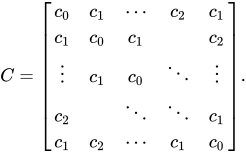
In linear algebra, a circulant matrix is a square matrix in which all rows are composed of the same elements and each row is rotated one element to the right relative to the preceding row. It is a particular kind of Toeplitz matrix.

In numerical analysis, circulant matrices are important because they are diagonalized by a discrete Fourier transform, and hence linear equations that contain them may be quickly solved using a fast Fourier transform.[1] They can be interpreted analytically as the integral kernel of a convolution operator on the cyclic group and hence frequently appear in formal descriptions of spatially invariant linear operations. This property is also critical in modern software defined radios, which utilize Orthogonal Frequency Division Multiplexing to spread the symbols (bits) using a cyclic prefix. This enables the channel to be represented by a circulant matrix, simplifying channel equalization in the frequency domain.

In cryptography, a circulant matrix is used in the MixColumns step of the Advanced Encryption Standard.

Definition

[edit]

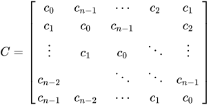
An circulant matrix takes the form or the transpose of this form (by choice of notation). If each is a square matrix, then the matrix is called a block-circulant matrix.

A circulant matrix is fully specified by one vector, , which appears as the first column (or row) of . The remaining columns (and rows, resp.) of are each cyclic permutations of the vector with offset equal to the column (or row, resp.) index, if lines are indexed from to . (Cyclic permutation of rows has the same effect as cyclic permutation of columns.) The last row of is the vector shifted by one in reverse.

Different sources define the circulant matrix in different ways, for example as above, or with the vector corresponding to the first row rather than the first column of the matrix; and possibly with a different direction of shift (which is sometimes called an anti-circulant matrix).

The polynomial is called the associated polynomial of the matrix .

Properties

[edit]

Eigenvectors and eigenvalues

[edit]

The normalized eigenvectors of a circulant matrix are the Fourier modes, namely, where is a primitive -th root of unity and is the imaginary unit.

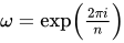
(This can be understood by realizing that multiplication with a circulant matrix implements a convolution. In Fourier space, convolutions become multiplication. Hence the product of a circulant matrix with a Fourier mode yields a multiple of that Fourier mode, i.e. it is an eigenvector.)

The corresponding eigenvalues are given by

Determinant

[edit]

As a consequence of the explicit formula for the eigenvalues above, the determinant of a circulant matrix can be computed as: Since taking the transpose does not change the eigenvalues of a matrix, an equivalent formulation is


Rank

[edit]

The rank of a circulant matrix is equal to where is the degree of the polynomial .[2]

Other properties

[edit]
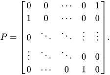
  • Any circulant is a matrix polynomial (namely, the associated polynomial) in the cyclic permutation matrix : where is given by the companion matrix
  • The set of circulant matrices forms an -dimensional vector space with respect to addition and scalar multiplication. This space can be interpreted as the space of functions on the cyclic group of order , , or equivalently as the group ring of .
  • Circulant matrices form a commutative algebra, since for any two given circulant matrices and , the sum is circulant, the product is circulant, and .
  • For a nonsingular circulant matrix , its inverse is also circulant. For a singular circulant matrix, its Moore–Penrose pseudoinverse is circulant.
  • The discrete Fourier transform matrix of order is defined as by

There are important connections between circulant matrices and the DFT matrices. In fact, it can be shown that where is the first column of . The eigenvalues of are given by the product . This product can be readily calculated by a fast Fourier transform.[3]

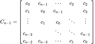
  • Let be the (monic) characteristic polynomial of an circulant matrix . Then the scaled derivative is the characteristic polynomial of the following submatrix of : (see [4] for the proof).

Analytic interpretation

[edit]

Circulant matrices can be interpreted geometrically, which explains the connection with the discrete Fourier transform.

Consider vectors in as functions on the integers with period , (i.e., as periodic bi-infinite sequences: ) or equivalently, as functions on the cyclic group of order (denoted or ) geometrically, on (the vertices of) the regular -gon: this is a discrete analog to periodic functions on the real line or circle.


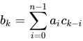
Then, from the perspective of operator theory, a circulant matrix is the kernel of a discrete integral transform, namely the convolution operator for the function ; this is a discrete circular convolution. The formula for the convolution of the functions is


(recall that the sequences are periodic) which is the product of the vector by the circulant matrix for .

The discrete Fourier transform then converts convolution into multiplication, which in the matrix setting corresponds to diagonalization.

The -algebra of all circulant matrices with complex entries is isomorphic to the group -algebra of

Symmetric circulant matrices

[edit]

For a symmetric circulant matrix one has the extra condition that . Thus it is determined by elements.

The eigenvalues of any real symmetric matrix are real. The corresponding eigenvalues become: for even, and for odd, where denotes the real part of . This can be further simplified by using the fact that and depending on even or odd.

Symmetric circulant matrices belong to the class of bisymmetric matrices.

Hermitian circulant matrices

[edit]

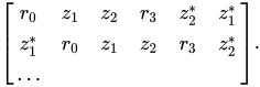
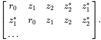
The complex version of the circulant matrix, ubiquitous in communications theory, is usually Hermitian. In this case and its determinant and all eigenvalues are real.

If n is even the first two rows necessarily takes the form in which the first element in the top second half-row is real.
If n is odd we get
Tee[5] has discussed constraints on the eigenvalues for the Hermitian condition.

Applications

[edit]

In linear equations

[edit]

Given a matrix equation

where is a circulant matrix of size , we can write the equation as the circular convolution where is the first column of , and the vectors , and are cyclically extended in each direction. Using the circular convolution theorem, we can use the discrete Fourier transform to transform the cyclic convolution into component-wise multiplication so that

This algorithm is much faster than the standard Gaussian elimination, especially if a fast Fourier transform is used.

In graph theory

[edit]

In graph theory, a graph or digraph whose adjacency matrix is circulant is called a circulant graph/digraph. Equivalently, a graph is circulant if its automorphism group contains a full-length cycle. The Möbius ladders are examples of circulant graphs, as are the Paley graphs for fields of prime order.

References

[edit]
[edit]
Revisions and contributorsEdit on WikipediaRead on Wikipedia
from Grokipedia
A circulant matrix is a square matrix in which each row vector is obtained by cyclically shifting the elements of the preceding row vector to the right by one position, with the first element wrapping around to the end.[1] For an n×nn \times n circulant matrix CC generated by the first row vector (c0,c1,,cn1)(c_0, c_1, \dots, c_{n-1}), the entry in the ii-th row and jj-th column is given by c(ji)modnc_{(j-i) \mod n}.[2] This structure makes circulant matrices a special subclass of Toeplitz matrices, characterized by constant values along their diagonals that wrap around due to the cyclic nature.[1] Circulant matrices possess several notable algebraic properties that distinguish them from general matrices. They form a commutative algebra under matrix multiplication, meaning the product of two circulant matrices is also circulant, and they commute with each other.[1] A key feature is their diagonalizability via the discrete Fourier transform (DFT): every circulant matrix CC can be expressed as C=F1ΛFC = F^{-1} \Lambda F, where FF is the unitary DFT matrix with entries Fk,l=n1/2ωklF_{k,l} = n^{-1/2} \omega^{kl} (ω=e2πi/n\omega = e^{-2\pi i / n}), and Λ\Lambda is a diagonal matrix containing the eigenvalues λm=k=0n1ckωmk,m=0,1,,n1\lambda_m = \sum_{k=0}^{n-1} c_k \omega^{mk}, \quad m = 0, 1, \dots, n-1, which are precisely the DFT of the generating vector.[1] This spectral decomposition simplifies computations such as inversion and exponentiation, as the eigenvalues allow efficient operations using fast Fourier transforms.[1] These matrices arise prominently in applications involving periodicity and convolution, such as digital signal processing, where they model circular convolution operations central to the DFT.[1] They also appear in coding theory for cyclic error-correcting codes, vibration analysis of periodic structures, and approximations of more general Toeplitz systems in numerical linear algebra.[1][3] Due to their symmetry, circulant matrices are normal and thus unitarily diagonalizable, facilitating their use in quantum computing and random matrix theory for modeling circulant ensembles.[4][5]

Definition and Examples

Definition

A circulant matrix is a square matrix in which each row is obtained by cyclically shifting the elements of the previous row to the right, with the shifted-out element wrapping around to the left end.[2] This structure arises from the concept of cyclic permutations, where the positions of elements cycle through a fixed order.[1] Formally, an n×nn \times n circulant matrix CC is generated by a vector c=(c0,c1,,cn1)\mathbf{c} = (c_0, c_1, \dots, c_{n-1}), with entries defined by Ci,j=c(ji)modnC_{i,j} = c_{(j - i) \mod n} for indices i,j=0,1,,n1i, j = 0, 1, \dots, n-1.[1] The modular arithmetic in the index ensures the cyclic wrap-around, distinguishing circulant matrices from more general forms. For instance, when n=3n=3 and c=(c0,c1,c2)\mathbf{c} = (c_0, c_1, c_2), the matrix takes the form
(c0c1c2c2c0c1c1c2c0). \begin{pmatrix} c_0 & c_1 & c_2 \\ c_2 & c_0 & c_1 \\ c_1 & c_2 & c_0 \end{pmatrix}.
[2] The concept of circulant matrices first appeared implicitly in the 1846 work of Eugène Catalan.[6] Circulant matrices represent a special case of Toeplitz matrices, where entries are constant along each diagonal, but enforced by the cyclic shifting.[1]

Examples

A circulant matrix is constructed by taking a generating vector and forming each subsequent row as a right cyclic shift of the previous row. For instance, consider a 2×2 circulant matrix generated by the vector $ (c_0, c_1) $. The matrix takes the form
(c0c1c1c0), \begin{pmatrix} c_0 & c_1 \\ c_1 & c_0 \end{pmatrix},
where the second row is the first row shifted right by one position, with the shifted element wrapping around to the beginning.[7] For a 3×3 example, let the generating vector be $ (1, 2, 3) $. The resulting circulant matrix is
(123312231), \begin{pmatrix} 1 & 2 & 3 \\ 3 & 1 & 2 \\ 2 & 3 & 1 \end{pmatrix},
illustrating the pattern where each row shifts the elements right cyclically from the row above. This cyclic structure is visually evident in the repetition of entries along wrap-around diagonals, emphasizing the matrix's Toeplitz-like but fully periodic nature.[7][2] Trivial cases include the zero circulant matrix, where the generating vector consists of all zeros, yielding an all-zero matrix that satisfies the cyclic shift property vacuously. The identity matrix is another boundary example, generated by $ (1, 0, 0, \dots, 0) $, placing 1s on the main diagonal and zeros elsewhere, with shifts preserving the diagonal structure.[7] Circulant permutation matrices arise as special cases where the generating vector has exactly one 1 and the rest zeros, corresponding to cyclic permutations. For $ n=3 $, the generating vector $ (0, 1, 0) $ produces the matrix
(010001100), \begin{pmatrix} 0 & 1 & 0 \\ 0 & 0 & 1 \\ 1 & 0 & 0 \end{pmatrix},
which represents a full cycle shift and is both circulant and a permutation matrix. The identity matrix serves as the case for the trivial cycle (no shift).[8]

Properties

Eigenvalues and Eigenvectors

Circulant matrices are normal and thus diagonalizable over the complex numbers, with their spectral decomposition relying on the discrete Fourier transform. Specifically, any n×nn \times n circulant matrix CC generated by the vector c=(c0,c1,,cn1)c = (c_0, c_1, \dots, c_{n-1}) can be expressed as C=FDF1C = F D F^{-1}, where FF is the Fourier matrix, DD is a diagonal matrix containing the eigenvalues of CC, and F1F^{-1} is the inverse Fourier matrix.[1][7] The eigenvectors of CC are the columns of the unitary Fourier matrix FF, whose entries are given by
Fj,k=ωjkn,j,k=0,1,,n1, F_{j,k} = \frac{\omega^{jk}}{\sqrt{n}}, \quad j,k = 0, 1, \dots, n-1,
where ω=e2πi/n\omega = e^{2\pi i / n} is the primitive nnth root of unity. This implies that all circulant matrices of order nn share the same eigenvectors, independent of the generating vector cc, due to the common eigenspaces formed by the Fourier basis vectors. The kkth eigenvector is thus v(k)=1n(1,ωk,ω2k,,ω(n1)k)Tv^{(k)} = \frac{1}{\sqrt{n}} (1, \omega^k, \omega^{2k}, \dots, \omega^{(n-1)k})^T.[1][7] The eigenvalues λk\lambda_k corresponding to these eigenvectors are the values of the discrete Fourier transform (DFT) of the generating vector cc:
λk=j=0n1cjωjk,k=0,1,,n1. \lambda_k = \sum_{j=0}^{n-1} c_j \omega^{jk}, \quad k = 0, 1, \dots, n-1.
Here, λk\lambda_k represents the kkth Fourier coefficient of cc, and the diagonal matrix D=diag(λ0,λ1,,λn1)D = \operatorname{diag}(\lambda_0, \lambda_1, \dots, \lambda_{n-1}) fully captures the spectrum of CC. This connection arises because the DFT diagonalizes circulant matrices, transforming the cyclic convolution implicit in their structure into pointwise multiplication in the frequency domain.[1][7] To derive this, consider the action of CC on an eigenvector v(k)v^{(k)}. The \ellth entry of Cv(k)C v^{(k)} is m=0n1c(m)modnvm(k)=1nm=0n1c(m)modnωmk\sum_{m=0}^{n-1} c_{(m - \ell) \mod n} v^{(k)}_m = \frac{1}{\sqrt{n}} \sum_{m=0}^{n-1} c_{(m - \ell) \mod n} \omega^{m k}. Let s=(m)modns = (m - \ell) \mod n; then m=(s+)modnm = (s + \ell) \mod n and ωmk=ωskωk\omega^{m k} = \omega^{s k} \omega^{\ell k}, so the sum becomes ωkns=0n1csωsk=λkv(k)\frac{\omega^{\ell k}}{\sqrt{n}} \sum_{s=0}^{n-1} c_s \omega^{s k} = \lambda_k v^{(k)}_\ell. This confirms Cv(k)=λkv(k)C v^{(k)} = \lambda_k v^{(k)} and leverages the shift-invariance of CC and the orthogonality of the Fourier basis.[7][1]

Determinant and Trace

The trace of an n×nn \times n circulant matrix CC generated by the vector (c0,c1,,cn1)(c_0, c_1, \dots, c_{n-1}) is the sum of its diagonal entries, all of which equal c0c_0, yielding Tr(C)=nc0\operatorname{Tr}(C) = n c_0.[1] This scalar invariant follows directly from the structure of circulant matrices, where each row is a right cyclic shift of the previous one, ensuring uniform diagonal elements.[9] The determinant of CC is the product of its eigenvalues: det(C)=k=0n1λk\det(C) = \prod_{k=0}^{n-1} \lambda_k, where the eigenvalues λk\lambda_k are given by the discrete Fourier transform of the generating vector, as derived from the spectral decomposition of circulant matrices.[1] Substituting the explicit form of the eigenvalues, λk=j=0n1cjωjk\lambda_k = \sum_{j=0}^{n-1} c_j \omega^{jk} with ω=e2πi/n\omega = e^{2\pi i / n} the primitive nnth root of unity, yields the closed-form expression
det(C)=k=0n1j=0n1cjωjk. \det(C) = \prod_{k=0}^{n-1} \sum_{j=0}^{n-1} c_j \omega^{jk}.
[9] This formula highlights the connection between the determinant and the roots of unity, facilitating efficient computation via the fast Fourier transform in practice.[1] A circulant matrix CC is singular if and only if det(C)=0\det(C) = 0, which occurs precisely when at least one eigenvalue λk=0\lambda_k = 0.[9] Equivalently, this happens if the associated polynomial p(z)=j=0n1cjzjp(z) = \sum_{j=0}^{n-1} c_j z^j evaluates to zero at some nnth root of unity ωk\omega^k, i.e., if pp shares a root with the nnth cyclotomic polynomial.[9] Such conditions provide insight into the invertibility of circulant matrices without requiring full spectral analysis.

Rank and Invertibility

The rank of an n×nn \times n circulant matrix CC, generated by the vector c=(c0,c1,,cn1)c = (c_0, c_1, \dots, c_{n-1}), is given by rank(C)=ndim(ker(C))\operatorname{rank}(C) = n - \dim(\ker(C)), where dim(ker(C))\dim(\ker(C)) equals the number of zero eigenvalues of CC, counting multiplicity.[1] Since CC is diagonalizable over the complex numbers via the Fourier matrix, the kernel dimension corresponds to the multiplicity of the zero eigenvalue.[1] The eigenvalues of CC are λk=p(ωk)\lambda_k = p(\omega^k) for k=0,1,,n1k = 0, 1, \dots, n-1, where ω\omega is a primitive nnth root of unity and p(x)=j=0n1cjxjp(x) = \sum_{j=0}^{n-1} c_j x^j is the associated generating polynomial.[1] Thus, dim(ker(C))\dim(\ker(C)) is the number of nnth roots of unity ωk\omega^k for which p(ωk)=0p(\omega^k) = 0, leading to rank deficiencies when p(x)p(x) shares roots with the nnth cyclotomic polynomial. For instance, consider the 2×22 \times 2 circulant matrix with first row [1,1][1, -1]; here p(x)=1xp(x) = 1 - x, so λ0=p(1)=0\lambda_0 = p(1) = 0 and λ1=p(1)=2\lambda_1 = p(-1) = 2, yielding dim(ker(C))=1\dim(\ker(C)) = 1 and rank(C)=1\operatorname{rank}(C) = 1. A circulant matrix CC is invertible if and only if all eigenvalues λk0\lambda_k \neq 0, which occurs precisely when the generating polynomial p(x)p(x) has no nth root of unity as a root.[10] In this case, dim(ker(C))=0\dim(\ker(C)) = 0 and rank(C)=n\operatorname{rank}(C) = n. When CC is invertible, its inverse C1C^{-1} is also a circulant matrix, generated by the vector whose entries are the inverse discrete Fourier transform of the sequence {1/λk}k=0n1\{1/\lambda_k\}_{k=0}^{n-1}.[1] Specifically, if FF denotes the unnormalized Fourier matrix with entries Fj,k=ωjkF_{j,k} = \omega^{jk}, then C=(1/n)FDFC = (1/n) F D F^*, where D=diag(λ0,,λn1)D = \operatorname{diag}(\lambda_0, \dots, \lambda_{n-1}), and C1=(1/n)FD1FC^{-1} = (1/n) F D^{-1} F^*, confirming the circulant structure.[1] Examples of rank deficiency arise when multiple eigenvalues vanish, such as in circulant matrices over finite fields where nilpotency conditions lead to partial nullity; for instance, certain circulant shift-like matrices modulo pp exhibit dim(ker(C))>0\dim(\ker(C)) > 0 without being the zero matrix. Over the complexes, however, non-trivial nilpotent circulant matrices do not exist, as all eigenvalues zero implies the generating polynomial is identically zero.

Additional Properties

The set of all n×nn \times n circulant matrices over a field forms a commutative subalgebra of the matrix algebra MnM_n, closed under addition, scalar multiplication, and matrix multiplication. Specifically, if CC and DD are circulant matrices generated by vectors c=(c0,c1,,cn1)\mathbf{c} = (c_0, c_1, \dots, c_{n-1}) and d=(d0,d1,,dn1)\mathbf{d} = (d_0, d_1, \dots, d_{n-1}), respectively, then C+DC + D is circulant with generating vector c+d\mathbf{c} + \mathbf{d}, αC\alpha C (for scalar α\alpha) is circulant with generating vector αc\alpha \mathbf{c}, and CD=DCCD = DC is circulant with generating vector given by the circular convolution of c\mathbf{c} and d\mathbf{d}.[1] The powers of a circulant matrix remain circulant. For a circulant matrix CC generated by c\mathbf{c}, the kk-th power CkC^k is circulant and generated by the vector obtained from the kk-fold circular convolution of c\mathbf{c} with itself. This follows from the closure under multiplication, as each successive product preserves the circulant structure.[1] Due to their shared eigensystem with the discrete Fourier transform matrix, all circulant matrices commute under multiplication, which underpins their formation of a commutative subalgebra. This commutativity distinguishes circulants from general matrices and facilitates simultaneous diagonalization.[1] The minimal polynomial of any n×nn \times n circulant matrix divides xn1x^n - 1. This arises from the cyclic shift structure, where circulants are polynomials in the basic circulant permutation matrix (the companion matrix of xn1x^n - 1), whose minimal polynomial is xn1x^n - 1.[11] Matrix-vector multiplication by a circulant matrix CC generated by c\mathbf{c} yields the circular convolution of c\mathbf{c} and the input vector v\mathbf{v}. Formally, if Cv=wC \mathbf{v} = \mathbf{w}, then wj=i=0n1civ(ji)modnw_j = \sum_{i=0}^{n-1} c_i v_{(j-i) \mod n} for j=0,,n1j = 0, \dots, n-1, embodying the periodic wrapping inherent to circulants.[7]

Representations and Interpretations

Polynomial Representation

A circulant matrix CC of order nn with first row entries c0,c1,,cn1c_0, c_1, \dots, c_{n-1} is associated with the polynomial p(x)=j=0n1cjxjC[x]p(x) = \sum_{j=0}^{n-1} c_j x^j \in \mathbb{C}[x].[12] This association arises because the matrix entries derive from the coefficients of p(x)p(x), and the cyclic shifts in subsequent rows correspond to the action of multiplying by powers of xx modulo xn1x^n - 1. Specifically, multiplication by xx in the ring C[x]/(xn1)\mathbb{C}[x]/(x^n - 1) cyclically shifts the coefficients of a polynomial, mirroring the row shifts in CC, so that CC represents multiplication by p(x)p(x) in this quotient ring.[1] The set of all n×nn \times n circulant matrices over C\mathbb{C} forms a commutative algebra under matrix addition and multiplication, which is isomorphic to the polynomial ring C[x]/(xn1)\mathbb{C}[x]/(x^n - 1).[12] Under this isomorphism, the standard basis matrix for the right shift (with 1 in the superdiagonal and bottom-left position) maps to the indeterminate xx, and every circulant matrix is the image of a unique polynomial of degree at most n1n-1. This structure preserves all algebraic operations, allowing circulant matrix computations to be performed equivalently in the polynomial ring.[1] The eigenvalues of CC are given by the evaluations λk=p(ωk)\lambda_k = p(\omega^k) for k=0,1,,n1k = 0, 1, \dots, n-1, where ω=e2πi/n\omega = e^{-2\pi i / n} is a primitive nnth root of unity.[1] This follows from the fact that the roots of unity filter the polynomial evaluations through the cyclic structure, yielding the spectrum directly from p(x)p(x). Equivalently, λk=j=0n1cjωjk\lambda_k = \sum_{j=0}^{n-1} c_j \omega^{j k}.[1]

Fourier Diagonalization

A key aspect of the structure of circulant matrices is their diagonalization via the Fourier matrix, which arises from the discrete Fourier transform (DFT). The unnormalized Fourier matrix $ F $ of order $ n $ is defined with entries $ F_{j,k} = \omega^{j k} $ for $ j, k = 0, 1, \dots, n-1 $, where $ \omega = e^{-2\pi i / n} $ is a primitive $ n $-th root of unity. This matrix satisfies $ F F^* = n I_n $, where $ F^* $ denotes the conjugate transpose, making its inverse $ F^{-1} = \frac{1}{n} F^* $.[1] The normalized Fourier matrix $ \hat{F} = n^{-1/2} F $ is unitary, satisfying $ \hat{F}^* \hat{F} = I_n $ and thus preserving the Euclidean norm in transformations. Every $ n \times n $ circulant matrix $ C $ admits the diagonalization $ C = \frac{1}{n} F D F^* $, where $ D $ is the diagonal matrix whose entries are the eigenvalues of $ C $. Equivalently, in unitary form, $ C = \hat{F} D \hat{F}^* $. These eigenvalues correspond to evaluations of the polynomial associated with the first row of $ C $ at the $ n $-th roots of unity.[1][13] This decomposition facilitates efficient numerical computations, as matrix-vector products involving $ C $ reduce to multiplications by $ F $, $ D $, and $ F^* $, which can be performed in $ O(n \log n) $ time using the fast Fourier transform (FFT) algorithm. The FFT exploits the recursive structure of the DFT to accelerate these operations, underpinning applications in numerical linear algebra.[1]

Special Types

Symmetric Circulant Matrices

A symmetric circulant matrix is a circulant matrix CC over the real numbers that is equal to its transpose, C=CTC = C^T. If CC is the n×nn \times n circulant matrix generated by the vector c=(c0,c1,,cn1)\mathbf{c} = (c_0, c_1, \dots, c_{n-1}), the symmetry condition requires that the generating vector be palindromic, satisfying cj=cnjc_j = c_{n-j} for all j=1,2,,n/2j = 1, 2, \dots, \lfloor n/2 \rfloor.[14] This ensures that each row is a right cyclic shift of the previous row while maintaining symmetry across the main diagonal.[7] Due to the symmetry, all eigenvalues of a symmetric circulant matrix are real numbers. The eigenvalues are given explicitly by
λk=c0+2j=1(n1)/2cjcos(2πkjn)+{(1)kcn/2if n even0otherwise \lambda_k = c_0 + 2 \sum_{j=1}^{\lfloor (n-1)/2 \rfloor} c_j \cos\left( \frac{2\pi k j}{n} \right) + \begin{cases} (-1)^k c_{n/2} & \text{if } n \text{ even} \\ 0 & \text{otherwise} \end{cases}
for k=0,1,,n1k = 0, 1, \dots, n-1.[14] The eigenvectors of CC are the same as those of any circulant matrix, namely the columns of the discrete Fourier transform matrix, but these are generally complex. However, real-valued eigenvectors can be formed by taking appropriate linear combinations of the real and imaginary parts of the Fourier eigenvectors, yielding an orthonormal basis that corresponds to the discrete cosine transform and discrete sine transform.[7][15] For example, consider the 3×3 symmetric circulant matrix generated by c=(2,1,1)\mathbf{c} = (2, 1, 1):
C=(211121112). C = \begin{pmatrix} 2 & 1 & 1 \\ 1 & 2 & 1 \\ 1 & 1 & 2 \end{pmatrix}.
This matrix has eigenvalues 4, 1, and 1, all real, with corresponding real eigenvectors including (1,1,1)T(1, 1, 1)^T for λ=4\lambda = 4 and vectors like (1,1/2,1/2)T(1, -1/2, -1/2)^T and (0,3/2,3/2)T(0, \sqrt{3}/2, -\sqrt{3}/2)^T for the degenerate eigenvalue 1 (up to scaling).[14] Symmetric circulant matrices represent a special subclass of symmetric Toeplitz matrices, where the wrap-around entries match the adjacent off-diagonals due to the palindromic structure, but their circulant nature enables efficient diagonalization via Fourier methods adapted for real bases.[16]

Hermitian Circulant Matrices

A Hermitian circulant matrix is a square matrix that is both circulant and Hermitian, meaning it equals its own conjugate transpose, $ C = C^H $. For an $ n \times n $ circulant matrix generated by the first row $ (c_0, c_1, \dots, c_{n-1}) $, the Hermitian condition requires $ c_j = \overline{c_{n-j}} $ for $ j = 0, 1, \dots, n-1 $, where the overline denotes complex conjugation; this ensures the diagonal entries are real and the off-diagonal entries satisfy conjugate symmetry.[7] The real-valued case, where all $ c_j $ are real, reduces to a symmetric circulant matrix. As a consequence of being Hermitian, all eigenvalues of a Hermitian circulant matrix are real. These eigenvalues are obtained via the discrete Fourier transform (DFT) of the generating row: $ \lambda_k = \sum_{j=0}^{n-1} c_j \omega^{j k} $ for $ k = 0, 1, \dots, n-1 $, where $ \omega = e^{2\pi i / n} $ is a primitive $ n $-th root of unity; the conjugate symmetry of the $ c_j $ guarantees the reality of each $ \lambda_k $.[7] Hermitian circulant matrices are normal and thus unitarily diagonalizable by the normalized Fourier matrix $ \frac{1}{\sqrt{n}} F $, where $ F_{j k} = \omega^{j k} $.[16] Such matrices arise in quantum computing for implementing dense operators efficiently via quantum circuits that exploit their circulant structure, and in signal processing for designing filters with cyclic symmetry properties.[17][1] A special case occurs when a Hermitian circulant matrix is unitary, satisfying $ C C^H = I $. In this scenario, since the matrix is both Hermitian and unitary, its eigenvalues must lie on the unit circle and be real, hence $ \lambda_k = \pm 1 $ for all $ k $; this implies $ C^2 = I $, making such matrices involutory.[7] A Hermitian circulant matrix is positive definite if all its eigenvalues satisfy $ \lambda_k > 0 $ for $ k = 0, 1, \dots, n-1 $. This holds if and only if the associated trigonometric polynomial $ p(\theta) = \sum_{j=0}^{n-1} c_j e^{i j \theta} $ is strictly positive for all $ \theta \in [0, 2\pi) $, as the eigenvalues are samples of $ p $ at equally spaced points on the unit circle.[7][1]

Applications

Solving Linear Systems

Solving linear systems involving circulant matrices offers significant computational advantages over general methods due to their diagonalization by the Fourier matrix. For a general n×nn \times n linear system Cx=bCx = b, where CC is an arbitrary matrix, direct methods like Gaussian elimination require O(n3)O(n^3) operations, which becomes prohibitive for large nn. In contrast, when CC is circulant, the system can be solved in O(nlogn)O(n \log n) time by exploiting the fast Fourier transform (FFT).[7] The efficient method leverages the Fourier diagonalization of circulant matrices, where C=FDF1C = F D F^{-1} with FF the DFT matrix and DD diagonal containing the eigenvalues of CC. To solve Cx=bCx = b, first compute the DFT of bb as b^=F1b\hat{b} = F^{-1} b, then divide componentwise by the eigenvalues to get x^=D1b^\hat{x} = D^{-1} \hat{b}, and finally recover x=Fx^x = F \hat{x} via the inverse DFT. Assuming CC is invertible, this process assumes access to the eigenvalues, which are themselves the DFT of the first column (or row) of CC. The FFT enables all transforms in O(nlogn)O(n \log n) time, with the division step costing O(n)O(n).[18] In standard notation with the unnormalized DFT matrix FF where Fjk=ωjkF_{jk} = \omega^{jk} and ω=e2πi/n\omega = e^{-2\pi i / n}, the solution formula is
x=1nF(D1(Fb)), x = \frac{1}{n} F \left( D^{-1} (F^* b) \right),
with FF^* the conjugate transpose of FF, since F1=F/nF^{-1} = F^* / n. This assumes CC is invertible, so all eigenvalues in DD are nonzero.[18]
Numerical stability of this approach depends on the conditioning of CC, which for normal matrices like circulants is determined by the ratio of the largest to smallest absolute eigenvalue, κ2(C)=maxiλi/miniλi\kappa_2(C) = \max_i |\lambda_i| / \min_i |\lambda_i|. A large eigenvalue spread amplifies relative errors in bb to errors in xx, particularly sensitive in the division step if eigenvalues are ill-conditioned. The FFT itself introduces rounding errors bounded by O(ϵnlogn)O(\epsilon n \log n) in floating-point arithmetic, where ϵ\epsilon is machine precision, but the overall error is dominated by the condition number when κ2(C)1\kappa_2(C) \gg 1.[1]

Graph Theory

In graph theory, a circulant graph is defined as an undirected graph with vertex set Zn\mathbb{Z}_n, the integers modulo nn, where two vertices ii and jj are adjacent if and only if ji±k(modn)j - i \equiv \pm k \pmod{n} for some kk in a symmetric subset SZn{0}S \subseteq \mathbb{Z}_n \setminus \{0\}, with SS closed under additive inverses. This construction ensures the graph's regularity and cyclic symmetry, making it a special case of a Cayley graph on the cyclic group Zn\mathbb{Z}_n.[19] The adjacency matrix of a circulant graph is a symmetric circulant matrix, where the entry in the first row at position kk is 1 if kSk \in S or kS-k \in S, and 0 otherwise, with subsequent rows obtained by cyclic shifts. This matrix structure reflects the graph's automorphism group, which includes the cyclic shifts ii+1(modn)i \mapsto i + 1 \pmod{n}, rendering all circulant graphs vertex-transitive. In spectral graph theory, the eigenvalues of this adjacency matrix are particularly tractable and given by the discrete Fourier transform of the first row: λj=sSexp(2πijs/n)\lambda_j = \sum_{s \in S} \exp(2\pi i j s / n) for j=0,1,,n1j = 0, 1, \dots, n-1, which, due to symmetry, yield real values expressible as sums of cosines.[19] These eigenvalues facilitate analysis of graph properties such as connectivity, expansion, and spectral gaps. Prominent examples include the cycle graph CnC_n, which arises when S={1,n1}S = \{1, n-1\} and represents the simplest non-trivial circulant graph with degree 2. The complete graph KnK_n is also circulant, obtained by taking S=Zn{0}S = \mathbb{Z}_n \setminus \{0\}, connecting every pair of distinct vertices and yielding the highest possible degree n1n-1.

Signal Processing

Circulant matrices play a fundamental role in signal processing, particularly in representing circular convolution operations essential for analyzing periodic signals. The product of a circulant matrix C\mathbf{C}, generated by its first row vector c\mathbf{c}, and an input vector v\mathbf{v} yields the circular convolution Cv=cv\mathbf{C} \mathbf{v} = \mathbf{c} * \mathbf{v}, where the convolution wraps around the signal boundaries to model periodicity. This structure is key in discrete-time signal processing for tasks involving cyclic data, such as audio looping or periodic noise analysis.[1][20] The efficiency of circular convolution is dramatically enhanced by the fast Fourier transform (FFT), leveraging the convolution theorem in the frequency domain. Specifically, the circular convolution equals the inverse discrete Fourier transform (IDFT) of the element-wise (Hadamard) product of the DFTs of the convolved sequences:
cv=F1(F(c)F(v)), \mathbf{c} * \mathbf{v} = \mathcal{F}^{-1} \left( \mathcal{F}(\mathbf{c}) \odot \mathcal{F}(\mathbf{v}) \right),
where F\mathcal{F} denotes the DFT and \odot the element-wise multiplication. This approach reduces the computational complexity from O(n2)O(n^2) for direct matrix-vector multiplication to O(nlogn)O(n \log n) using the FFT algorithm, making it indispensable for real-time signal processing applications like spectral filtering.[1][20] In finite impulse response (FIR) filter design, circulant matrices approximate the Toeplitz matrices that arise in linear convolution, enabling fast implementation via FFT-based methods. By zero-padding the input signal and filter coefficients to a sufficient length, the linear convolution can be exactly represented as a circular one, avoiding wrap-around artifacts and facilitating efficient FIR filtering in systems like digital audio equalizers.[1] The Toeplitz-circulant approximation extends this utility to non-circular scenarios, where the banded Toeplitz matrix of a linear filter is closely approximated by a circulant matrix for large signal dimensions, with eigenvalues converging asymptotically. This technique, though rooted in early literature, remains relevant for preconditioning in iterative solvers and approximating filter responses in oversized convolutions.[1]

Other Fields

In coding theory, cyclic codes, including BCH codes, can be generated using circulant matrices derived from the generator polynomial, where the matrix rows are cyclic shifts of the polynomial coefficients, facilitating efficient encoding and error correction via polynomial ideals in the ring Z[x]/(xn1)\mathbb{Z}[x]/(x^n - 1).[21] Specifically, for BCH codes, circulant matrices enable the construction of parity-check matrices and support decoding algorithms like Berlekamp-Massey, which exploit the spectral properties of circulants for minimum distance bounds.[21] In cryptography, circulant matrices underpin lattice-based schemes such as NTRU, where polynomial multiplication in the quotient ring Z[x]/(xN1)\mathbb{Z}[x]/(x^N - 1) corresponds to multiplication by a circulant public key matrix AA, enabling fast encryption and decryption through cyclic convolutions.[22] This structure provides resistance to lattice reduction attacks while maintaining computational efficiency.[22] In combinatorics, the enumeration of circulant matrices often focuses on special classes, such as binary or ±1\pm 1-entry matrices satisfying orthogonality conditions.[23] Hadamard matrices serve as a notable special case, with the circulant Hadamard conjecture positing that the only such matrices exist for orders 1 and 4, as verified for small orders and supported by eigenvalue constraints.[24] Recent developments in quantum computing leverage circulant matrices for efficient simulations, particularly in algorithms for matrix-vector multiplication that achieve exponential speedup over classical methods, aiding applications like quantum convolutional neural networks.[25] For instance, post-2020 quantum circuits compute circulant products in O(logN)O(\log N) time for real entries, enhancing simulation of periodic systems without relying on full Hamiltonian oracle queries.[25]
User Avatar
No comments yet.