Recent from talks
Contribute something
Nothing was collected or created yet.
Geodynamics
View on Wikipedia| Part of a series of |
| Geophysics |
|---|
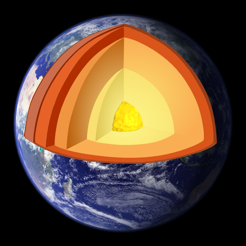
Geodynamics is a subfield of geophysics dealing with dynamics of the Earth. It applies physics, chemistry and mathematics to the understanding of how mantle convection leads to plate tectonics and geologic phenomena such as seafloor spreading, mountain building, volcanoes, earthquakes, or faulting. It also attempts to probe the internal activity by measuring magnetic fields, gravity, and seismic waves, as well as the mineralogy of rocks and their isotopic composition. Methods of geodynamics are also applied to exploration of other planets.[1]
Overview
[edit]Geodynamics is generally concerned with processes that move materials throughout the Earth. In the Earth's interior, movement happens when rocks melt or deform and flow in response to a stress field.[2] This deformation may be brittle, elastic, or plastic, depending on the magnitude of the stress and the material's physical properties, especially the stress relaxation time scale. Rocks are structurally and compositionally heterogeneous and are subjected to variable stresses, so it is common to see different types of deformation in close spatial and temporal proximity.[3] When working with geological timescales and lengths, it is convenient to use the continuous medium approximation and equilibrium stress fields to consider the average response to average stress.[4]
Experts in geodynamics commonly use data from geodetic GPS, InSAR, and seismology, along with numerical models, to study the evolution of the Earth's lithosphere, mantle and core.
Work performed by geodynamicists may include:
- Modeling brittle and ductile deformation of geologic materials
- Predicting patterns of continental accretion and breakup of continents and supercontinents
- Observing surface deformation and relaxation due to ice sheets and post-glacial rebound, and making related conjectures about the viscosity of the mantle
- Finding and understanding the driving mechanisms behind plate tectonics.
Deformation of rocks
[edit]Rocks and other geological materials experience strain according to three distinct modes, elastic, plastic, and brittle depending on the properties of the material and the magnitude of the stress field. Stress is defined as the average force per unit area exerted on each part of the rock. Pressure is the part of stress that changes the volume of a solid; shear stress changes the shape. If there is no shear, the fluid is in hydrostatic equilibrium. Since, over long periods, rocks readily deform under pressure, the Earth is in hydrostatic equilibrium to a good approximation. The pressure on rock depends only on the weight of the rock above, and this depends on gravity and the density of the rock. In a body like the Moon, the density is almost constant, so a pressure profile is readily calculated. In the Earth, the compression of rocks with depth is significant, and an equation of state is needed to calculate changes in density of rock even when it is of uniform composition.[5]
Elastic
[edit]Elastic deformation is always reversible, which means that if the stress field associated with elastic deformation is removed, the material will return to its previous state. Materials only behave elastically when the relative arrangement along the axis being considered of material components (e.g. atoms or crystals) remains unchanged. This means that the magnitude of the stress cannot exceed the yield strength of a material, and the time scale of the stress cannot approach the relaxation time of the material. If stress exceeds the yield strength of a material, bonds begin to break (and reform), which can lead to ductile or brittle deformation.[6]
Ductile
[edit]Ductile or plastic deformation happens when the temperature of a system is high enough so that a significant fraction of the material microstates (figure 1) are unbound, which means that a large fraction of the chemical bonds are in the process of being broken and reformed. During ductile deformation, this process of atomic rearrangement redistributes stress and strain towards equilibrium faster than they can accumulate.[6] Examples include bending of the lithosphere under volcanic islands or sedimentary basins, and bending at oceanic trenches.[5] Ductile deformation happens when transport processes such as diffusion and advection that rely on chemical bonds to be broken and reformed redistribute strain about as fast as it accumulates.
Brittle
[edit]When strain localizes faster than these relaxation processes can redistribute it, brittle deformation occurs. The mechanism for brittle deformation involves a positive feedback between the accumulation or propagation of defects especially those produced by strain in areas of high strain, and the localization of strain along these dislocations and fractures. In other words, any fracture, however small, tends to focus strain at its leading edge, which causes the fracture to extend.[6]
In general, the mode of deformation is controlled not only by the amount of stress, but also by the distribution of strain and strain associated features. Whichever mode of deformation ultimately occurs is the result of a competition between processes that tend to localize strain, such as fracture propagation, and relaxational processes, such as annealing, that tend to delocalize strain.
Deformation structures
[edit]Structural geologists study the results of deformation, using observations of rock, especially the mode and geometry of deformation to reconstruct the stress field that affected the rock over time. Structural geology is an important complement to geodynamics because it provides the most direct source of data about the movements of the Earth. Different modes of deformation result in distinct geological structures, e.g. brittle fracture in rocks or ductile folding.
Thermodynamics
[edit]The physical characteristics of rocks that control the rate and mode of strain, such as yield strength or viscosity, depend on the thermodynamic state of the rock and composition. The most important thermodynamic variables in this case are temperature and pressure. Both of these increase with depth, so to a first approximation the mode of deformation can be understood in terms of depth. Within the upper lithosphere, brittle deformation is common because under low pressure rocks have relatively low brittle strength, while at the same time low temperature reduces the likelihood of ductile flow. After the brittle-ductile transition zone, ductile deformation becomes dominant.[2] Elastic deformation happens when the time scale of stress is shorter than the relaxation time for the material. Seismic waves are a common example of this type of deformation. At temperatures high enough to melt rocks, the ductile shear strength approaches zero, which is why shear mode elastic deformation (S-Waves) will not propagate through melts.[7]
Forces
[edit]The main motive force behind stress in the Earth is provided by thermal energy from radioisotope decay, friction, and residual heat.[8][9] Cooling at the surface and heat production within the Earth create a metastable thermal gradient from the hot core to the relatively cool lithosphere.[10] This thermal energy is converted into mechanical energy by thermal expansion. Deeper and hotter rocks often have higher thermal expansion and lower density relative to overlying rocks. Conversely, rock that is cooled at the surface can become less buoyant than the rock below it. Eventually this can lead to a Rayleigh-Taylor instability (Figure 2), or interpenetration of rock on different sides of the buoyancy contrast.[2][11]

Negative thermal buoyancy of the oceanic plates is the primary cause of subduction and plate tectonics,[12] while positive thermal buoyancy may lead to mantle plumes, which could explain intraplate volcanism.[13] The relative importance of heat production vs. heat loss for buoyant convection throughout the whole Earth remains uncertain and understanding the details of buoyant convection is a key focus of geodynamics.[2]
Methods
[edit]Geodynamics is a broad field which combines observations from many different types of geological study into a broad picture of the dynamics of Earth. Close to the surface of the Earth, data includes field observations, geodesy, radiometric dating, petrology, mineralogy, drilling boreholes and remote sensing techniques. However, beyond a few kilometers depth, most of these kinds of observations become impractical. Geologists studying the geodynamics of the mantle and core must rely entirely on remote sensing, especially seismology, and experimentally recreating the conditions found in the Earth in high pressure high temperature experiments.(see also Adams–Williamson equation).
Numerical modeling
[edit]Because of the complexity of geological systems, computer modeling is used to test theoretical predictions about geodynamics using data from these sources.
There are two main ways of geodynamic numerical modeling.[14]
- Modelling to reproduce a specific observation: This approach aims to answer what causes a specific state of a particular system.
- Modelling to produce basic fluid dynamics: This approach aims to answer how a specific system works in general.
Basic fluid dynamics modelling can further be subdivided into instantaneous studies, which aim to reproduce the instantaneous flow in a system due to a given buoyancy distribution, and time-dependent studies, which either aim to reproduce a possible evolution of a given initial condition over time or a statistical (quasi) steady-state of a given system.
See also
[edit]- Computational Infrastructure for Geodynamics – Organization that advances Earth science
- Cytherodynamics
References
[edit]- ^ Ismail-Zadeh & Tackley 2010
- ^ a b c d Turcotte, D. L. and G. Schubert (2014). "Geodynamics."
- ^ Winters, J. D. (2001). "An introduction to igenous and metamorphic petrology."
- ^ Newman, W. I. (2012). Continuum Mechanics in the Earth Sciences. Cambridge University Press. ISBN 9780521562898.
- ^ a b Turcotte & Schubert 2002
- ^ a b c Karato, Shun-ichiro (2008). "Deformation of Earth Materials: An Introduction to the Rheology of Solid Earth."
- ^ Faul, U. H., J. D. F. Gerald and I. Jackson (2004). "Shear wave attenuation and dispersion in melt-bearing olivine
- ^ Hager, B. H. and R. W. Clayton (1989). "Constraints on the structure of mantle convection using seismic observations, flow models, and the geoid." Fluid Mechanics of Astrophysics and Geophysics 4.
- ^ Stein, C. (1995). "Heat flow of the Earth."
- ^ Dziewonski, A. M. and D. L. Anderson (1981). "Preliminary reference Earth model." Physics of the Earth and Planetary Interiors 25(4): 297–356.
- ^ Ribe, N. M. (1998). "Spouting and planform selection in the Rayleigh–Taylor instability of miscible viscous fluids." Journal of Fluid Mechanics 377: 27–45.
- ^ Conrad, C. P. and C. Lithgow-Bertelloni (2004). "The temporal evolution of plate driving forces: Importance of "slab suction" versus "slab pull" during the Cenozoic." Journal of Geophysical Research 109(B10): 2156–2202.
- ^ Bourdon, B., N. M. Ribe, A. Stracke, A. E. Saal and S. P. Turner (2006). "Insights into the dynamics of mantle plumes from uranium-series geochemistry." Nature 444(7): 713–716.
- ^ Tackley, Paul J.; Xie, Shunxing; Nakagawa, Takashi; Hernlund, John W. (2005), "Numerical and laboratory studies of mantle convection: Philosophy, accomplishments, and thermochemical structure and evolution", Earth's Deep Mantle: Structure, Composition, and Evolution, vol. 160, American Geophysical Union, pp. 83–99, Bibcode:2005GMS...160...83T, doi:10.1029/160gm07, ISBN 9780875904252
- Bibliography
- Ismail-Zadeh, Alik; Tackley, Paul J. (2010). Computational methods for geodynamics. Cambridge University Press. ISBN 9780521867672.
- Jolivet, Laurent; Nataf, Henri-Claude; Aubouin, Jean (1998). Geodynamics. Taylor & Francis. ISBN 9789058092205.
- Turcotte, D.; Schubert, G. (2002). Geodynamics (2nd ed.). New York: Cambridge University Press. ISBN 978-0-521-66186-7.
External links
[edit]Geodynamics
View on GrokipediaIntroduction
Definition and Scope
Geodynamics is the study of the dynamic processes and physical forces that shape Earth's interior and surface, focusing on the mechanisms driving deformation, flow, and the overall evolution of its structure. It integrates principles from physics, mathematics, chemistry, geology, geophysics, and planetary science to provide a quantitative understanding of these phenomena.[5][6][7] The scope of geodynamics encompasses a vast range of spatial scales, from microscopic deformations in rocks at the centimeter level to planetary-scale motions involving the entire Earth, with particular emphasis on the dynamics of the mantle and lithosphere. It addresses temporal scales spanning seconds for seismic events to billions of years for major evolutionary changes, contrasting with human timescales by operating primarily over geological epochs. This field distinguishes itself from static geology, which focuses on structural descriptions without emphasizing ongoing motions, and from pure seismology, which centers on wave propagation during earthquakes, by prioritizing the modeling of time-dependent forces and flows.[5][6][7] Central to geodynamics is its role in elucidating Earth's thermal evolution, from ancient regimes to modern plate tectonics, which regulates heat loss through processes like mantle convection—the primary driver of material circulation and surface expressions such as volcanism. These dynamics also contribute to planetary habitability by influencing the carbon cycle, climate stability, and the maintenance of liquid water on the surface. A key application is plate tectonics, which explains the movement and interaction of lithospheric plates, shaping global geography and geological activity.[5][8][9][7]Historical Development
The concept of geodynamics emerged from early 20th-century geological observations, with Alfred Wegener's 1912 proposal of continental drift marking a foundational precursor. Wegener suggested that continents were once joined in a supercontinent called Pangaea and had since drifted apart, based on matching fossils, rock formations, and paleoclimatic evidence across the Atlantic.[10] However, his theory faced widespread rejection due to the lack of a plausible driving mechanism and insufficient evidence for continental movement over oceanic crust.[11] Arthur Holmes advanced these ideas in the 1920s and 1930s by integrating radioactivity as a heat source for Earth's interior, proposing mantle convection as the driving force for continental drift. In his 1928 lecture and subsequent works, Holmes described thermal convection currents in the mantle, driven by radioactive decay, as capable of dragging continents across the globe like conveyor belts.[12] His 1944 textbook further elaborated this mechanism, linking it to volcanic activity and orogeny, though it remained marginalized until mid-century evidence accumulated.[11] The revival of these concepts accelerated in the 1960s with the development of plate tectonics theory, independently formulated by Dan McKenzie, Robert L. Parker, and W. Jason Morgan. McKenzie and Parker's 1967 paper demonstrated that rigid lithospheric plates could move on a spherical Earth using Euler's theorem, fitting earthquake and magnetic data from the North Pacific. Morgan's 1968 work expanded this globally, identifying about a dozen major plates bounded by rises, trenches, and faults, with motions driven by mantle forces.[13] By the 1970s, seafloor spreading and subduction evidence solidified plate tectonics, while 1980s models incorporated mantle convection more rigorously, linking slab pull and ridge push to observed plate velocities.[14] Post-2000 advances in geodynamics integrated high-resolution seismology, geodesy, and computational modeling to refine these frameworks. Seismic tomography revealed mantle heterogeneity and plume structures, validating convection patterns.[15] Satellite-based GPS, operational since the 1990s, provided precise measurements of plate motions and deformation, confirming models at millimeter accuracy and enabling real-time monitoring of tectonic strain.[16] Numerical simulations, enhanced by supercomputing, now simulate whole-mantle dynamics, incorporating thermodynamics to predict long-term evolution.[17]Fundamental Principles
Thermodynamics
Thermodynamics governs the energy balance and material behavior within Earth's interior, providing the foundational principles for understanding geodynamic processes. The first law of thermodynamics, which states that energy is conserved, applies to Earth systems by accounting for the total internal energy as the sum of heat added, work done, and changes in stored energy forms such as thermal and gravitational potential.[18] In the mantle, this law balances heat inputs from various sources against losses primarily through conduction and convection at the surface, ensuring no net creation or destruction of energy over geological timescales. The second law introduces the concept of entropy, dictating that irreversible processes, such as viscous dissipation in flowing mantle material, increase the total entropy of the system, driving the Earth toward equilibrium while sustaining dynamic flows like convection.[19] The primary heat sources powering Earth's geodynamic engine include primordial heat retained from planetary accretion and core differentiation, radiogenic decay of isotopes like uranium-238, thorium-232, and potassium-40, and latent heat released during phase changes and inner core solidification. Primordial heat, estimated to contribute about 50% of the current heat budget (with recent models indicating ~25 TW non-radiogenic out of a total surface heat flux of 46 ± 3 TW as of 2022), originates from gravitational energy during formation approximately 4.54 billion years ago, while radiogenic heat dominates the mantle's ongoing production at roughly 15-20 terawatts.[20][21] Latent heat from exothermic phase transitions, such as the olivine to wadsleyite transformation at around 410 km depth, provides additional localized heating that influences convective vigor by releasing energy equivalent to several gigawatts per cubic kilometer during slab descent.[22] These sources collectively sustain a surface heat flux of about 47 terawatts, with the core-mantle boundary contributing significantly to the total budget. Key thermodynamic equations describe heat transport and temperature profiles in the mantle. The heat equation for thermal diffusion, , where is temperature, is time, and is thermal diffusivity (typically 10^{-6} m²/s for mantle rocks), governs conductive heat flow in regions of low convection, such as thermal boundary layers.[23] For ascending mantle material in adiabatic conditions, the temperature gradient follows , with as the thermal expansivity (about 2-3 × 10^{-5} K^{-1}), as gravitational acceleration (9.8 m/s²), and as specific heat capacity (around 1000 J/kg·K), yielding gradients of 0.3-0.5 K/km that prevent excessive cooling during upwelling.[24] In convective systems, entropy production arises from irreversible processes like shear heating and thermal diffusion, quantified as the rate of entropy increase , where is the stress tensor and is velocity, ensuring compliance with the second law by nonnegative values that quantify dissipative losses.[19] Phase transitions, exemplified by the exothermic olivine-wadsleyite boundary at 410 km, release latent heat that locally boosts entropy production and modulates convective instabilities by altering buoyancy.[22] Thermal boundary layers, typically 50-100 km thick at the lithosphere and core-mantle boundary, form where conduction dominates over advection, creating steep temperature gradients (up to 10-20 K/km) that separate the convecting interior from rigid boundaries.[25] Thermodynamic constraints limit Earth's cooling rate to about 100 K per billion years, consistent with its 4.54 billion-year age derived from radiometric dating of meteorites and lunar samples, allowing gradual heat loss while maintaining a hot interior.[21] These principles drive instabilities such as Rayleigh-Bénard convection, where thermal gradients exceed a critical Rayleigh number (Ra ≈ 10^3 for simple fluids, higher for viscous mantles), initiating buoyancy-driven flows that transport heat efficiently from the interior.[26] Mantle convection, as a thermodynamically driven process, exemplifies how entropy maximization organizes large-scale circulation despite viscous resistance.[23]Rheology of Earth Materials
Rheology describes the deformation and flow behavior of Earth materials under applied stress, which is fundamental to understanding geodynamic processes such as mantle convection and plate tectonics.[27] In the Earth's interior, rocks and minerals exhibit a range of rheological responses depending on temperature, pressure, strain rate, and composition, transitioning from brittle failure in the cold, shallow lithosphere to ductile flow in the warmer mantle.[28] Rheological models simplify these behaviors into mathematical frameworks, distinguishing between linear viscous flow, where strain rate is directly proportional to stress, and nonlinear behaviors dominated by mechanisms like dislocation creep.[29] Linear rheology, often modeled as Newtonian viscosity, applies to low-stress regimes where viscous flow occurs without significant microstructural changes, characterized by the relation , with as viscosity, as deviatoric shear stress, and as strain rate.[27] Nonlinear rheology predominates in the mantle, particularly through power-law creep associated with dislocation mechanisms, where strain rate follows , with as a material constant, as the stress exponent (typically 3-5 for dislocation creep), as activation energy, as the gas constant, and as temperature; this leads to an effective viscosity that decreases nonlinearly with increasing stress.[30] Temperature dependence in these models is captured by the Arrhenius relation , reflecting thermally activated processes like diffusion or dislocation motion, which link rheological properties to thermodynamic controls on atomic-scale diffusion. In the asthenosphere, a low-viscosity zone beneath the lithosphere, effective viscosities range around Pa·s, enabling ductile flow and decoupling of tectonic plates, while the overlying lithosphere behaves as an elastic-brittle shell with higher effective strength due to cooler temperatures.[31] Pressure generally increases viscosity by raising activation energies, but temperature exerts a stronger inverse effect, promoting flow in deeper, hotter regions; volatiles like water further weaken materials, as seen in quartz-rich crustal rocks where hydrolytic weakening reduces strength by orders of magnitude through enhanced dislocation mobility at hydroxyl concentrations as low as 100-1000 H/Si per formula unit.[32] For instance, water incorporation in quartz lattices lowers the activation energy for dislocation creep from about 220 kJ/mol in dry conditions to 140 kJ/mol in wet ones, facilitating deformation at shallower depths.[33] Rheological transitions define layer boundaries, such as the brittle-ductile transition at depths of 10-20 km in continental crust, where temperatures reach 250-400°C, shifting from frictional sliding to crystal-plastic flow based on strain rate and lithology.[34] In the olivine-rich upper mantle, rheological anisotropy arises from lattice-preferred orientation of olivine crystals during deformation, with slip systems like (010)[35] dominating at high stresses, leading to up to 50% variation in viscosity between directions and influencing seismic anisotropy patterns.[36] This anisotropy, combined with power-law creep, allows for localized shear zones in the mantle, as observed in dislocation-dominated flow regimes where for dry olivine.[29]Driving Forces
Internal Forces
Internal forces in geodynamics refer to endogenic mechanisms originating from density variations within Earth's interior that propel tectonic motions, primarily through gravitational instabilities. These forces arise from thermal contrasts that induce buoyancy effects, governed by Archimedes' principle, where less dense materials ascend and denser ones descend in the mantle. Mantle convection, driven by internal heating, generates these density differences via thermal expansion, creating upwellings and downwellings that interact with the lithosphere.[37] A key internal force is buoyancy, particularly in the mantle where thermal expansion reduces the density of heated material, leading to upward motion. The buoyancy force on a volume of material with density (lighter parcel) surrounded by mantle density is given by where is gravitational acceleration; this force drives convective circulation by countering the weight of denser surrounding rock.[37] In subduction zones, the converse applies: cold, dense oceanic slabs exhibit negative buoyancy, pulling the lithosphere downward with a slab pull force estimated at approximately to N/m along the trench.[38] This process releases gravitational potential energy as the slab sinks, providing the primary energy source for plate motion, with the potential energy per unit area quantified by the density contrast and descent depth.[37] Another significant internal force is ridge push, resulting from gravitational sliding of lithosphere away from elevated mid-ocean ridges, where buoyant, thickened crust creates a topographic gradient; this force magnitudes around N/m.[39] Mantle drag, or basal traction, arises from viscous coupling between the flowing asthenosphere and the lithosphere base, exerting shear stresses that can either resist or assist motion depending on flow direction, typically on the order of to N/m.[40] In the overall force balance of plate tectonics, slab pull dominates, accounting for about 60% of driving forces, while ridge push and mantle drag contribute lesser but complementary roles, together generating lithospheric stresses that influence faulting and deformation.[41]Surface and External Forces
Surface and external forces in geodynamics refer to those originating from or acting upon the Earth's exterior, including gravitational interactions with celestial bodies and surface mass redistributions, which perturb the lithosphere and influence tectonic processes. These forces are generally subordinate to internal drivers but can modulate stress fields, trigger localized deformation, and contribute to observable crustal movements. Unlike deep-seated buoyancy forces, surface and external forces operate at the lithosphere-atmosphere-ocean interface, often through loading and unloading mechanisms that alter local isostatic balance.[42] Tidal forces, primarily from the Moon and Sun, induce periodic deformations in the solid Earth, with magnitudes on the order of 10^11 N acting across tectonic plates due to differential gravitational pulls. These forces generate tidal stresses of approximately 0.1–10 kPa, which are minuscule compared to typical tectonic stress drops of 1–50 MPa but sufficient to influence seismicity in susceptible regions. The tidal potential perturbation is described by the quadrupolar component of the gravitational field, given by where is the gravitational constant, is the mass of the perturbing body (Moon or Sun), is the distance to the body, is the radial distance from Earth's center, and is the Legendre polynomial of degree 2; this potential drives elastic and anelastic responses in the lithosphere.[43][42] Another significant surface force arises from post-glacial isostatic rebound, where the removal of ice sheet loads following the Last Glacial Maximum causes ongoing uplift in formerly glaciated regions. In Fennoscandia, for example, global positioning system (GPS) measurements indicate uplift rates of approximately 1 cm per year in the Bothnian Bay, reflecting the viscoelastic relaxation of the mantle beneath the Scandinavian Shield. This adjustment is governed by the viscous relaxation time , where is the mantle viscosity (typically 10^{21} Pa·s), is the density of the deforming layer, is gravitational acceleration, and is the thickness of the layer; for upper mantle conditions, ranges from thousands to tens of thousands of years, allowing gradual rebound. Such rebound exemplifies isostasy as a response to surface unloading, redistributing stresses across continental interiors.[44][45] Interactions between surface processes and crustal loading further amplify external influences on geodynamics. Erosion removes mass from elevated terrains, reducing overburden and inducing extensional stresses in the upper crust, while sedimentation in adjacent basins adds load, promoting subsidence and compressional regimes; these effects can alter rift dynamics and basin evolution over geological timescales. Similarly, atmospheric and oceanic loading—through pressure variations and water mass redistribution—impose dynamic stresses on intraplate regions, with hydrological cycles contributing to annual-scale perturbations of up to several kPa that correlate with microseismicity in stable continental interiors like the New Madrid Seismic Zone. These loadings perturb the lithospheric stress field, potentially biasing brittle deformation along pre-existing faults.[46][47] Modern observations highlight the measurable impacts of these forces. GPS data from co-seismic events reveal that tidal loading can modulate slip magnitudes, with perturbations aligning seismic activity peaks during high-tide phases, as seen in correlations between tidal stress and earthquake nucleation durations. Overall, external forces contribute less than 5% to global plate motions, serving primarily as modulators rather than primary drivers, though they play a critical role in fine-tuning intraplate stress accumulation.[42]Deformation Mechanisms
Elastic Deformation
Elastic deformation refers to the reversible response of rocks to applied stress, where the material returns to its original shape upon stress removal, provided the stress remains below the elastic limit. This behavior is fundamental in geodynamics, governing short-term crustal responses to tectonic forces and the propagation of seismic waves. In rocks, elastic deformation arises from interatomic bonding forces that resist distortion, allowing strain to accumulate elastically until a threshold is reached.[48] The primary principle describing this process is Hooke's law, which relates stress to strain through the material's stiffness: , where is Young's modulus. For crustal rocks, typically ranges from 10 to 100 GPa, reflecting variations in mineral composition and microstructure.[49] This linear relation holds for small strains, enabling rocks to store elastic energy that can be released rapidly. Poisson's ratio , typically 0.2–0.3 for most rocks, quantifies the lateral contraction accompanying axial extension, influencing volumetric changes under stress.[50] In seismic wave propagation, stress-strain relations underpin the elastic wave equation, derived from Hooke's law and Newton's second law, which describes how P-waves and S-waves travel through the Earth at velocities dependent on elastic moduli. These relations ensure that wave speeds in crustal rocks, often 5–7 km/s for P-waves, reflect the elastic properties without permanent alteration.[51] A key geodynamic application is the elastic rebound theory, proposed by Harry Fielding Reid following the 1906 San Francisco earthquake, which explains how tectonic strain accumulates elastically across faults until sudden release during rupture. This process drives elastic strain accumulation over interseismic periods, building stress that is relieved in earthquakes, with global examples like the San Andreas Fault illustrating cycles of locking and slip.[52] Elastic deformation operates on short time scales, from seconds during wave passage to years in tectonic loading, distinguishing it as the initial response before viscoelastic effects dominate. In earthquakes, this accumulation enables forecasting potential energy release, as observed in subduction zones where interseismic strain builds at rates of millimeters per year.[53] Elastic properties in rocks often exhibit anisotropy due to mineral alignment; for instance, quartz crystals show direction-dependent stiffness, with elastic moduli varying up to 20% along different crystallographic axes, affecting localized stress distribution in the crust.[54] The elastic limit, or yield strength, marks the transition to plastic deformation, typically at differential stresses of 100–500 MPa for crustal rocks under ambient conditions, beyond which permanent strain occurs. GPS observations in subduction zones, such as the Japan Trench, reveal elastic plate bending with trenchward velocities of 5–8 cm/year, confirming reversible deformation in the overriding plate during interseismic phases.[55]Ductile Deformation
Ductile deformation refers to the permanent, time-dependent reshaping of rocks through viscous or plastic flow without fracturing, occurring primarily under elevated temperatures and pressures where interatomic bonds can rearrange. This process dominates in the Earth's deeper crust and mantle, enabling large-scale geodynamic movements such as convection and mountain building.[56] The primary mechanisms of ductile deformation in rocks are diffusion creep and dislocation creep. Diffusion creep involves the net migration of atoms or vacancies through the crystal lattice or along grain boundaries, driven by stress gradients, leading to homogeneous deformation without significant strain localization. Nabarro-Herring creep, a volume diffusion variant, occurs when atoms diffuse through the interiors of grains, while Coble creep relies on faster grain-boundary diffusion; both are Newtonian (linearly stress-dependent) and highly sensitive to grain size, with smaller grains enhancing creep rates due to shorter diffusion paths.[57][56] In contrast, dislocation creep arises from the glide and climb of dislocations within crystals, allowing non-linear, power-law strain rates that increase rapidly with stress; this mechanism produces lattice-preferred orientations (LPO) in minerals like olivine, contributing to seismic anisotropy observed in the mantle.[58] Grain size plays a critical role in the transition between these mechanisms, as diffusion creep dominates in fine-grained rocks (e.g., <10–100 μm for olivine), while dislocation creep prevails in coarser aggregates, influencing overall rock viscosity and flow localization in shear zones.[56] Ductile deformation typically initiates at depths greater than 20 km and temperatures exceeding 500°C, where geothermal gradients and confining pressures suppress brittle failure, allowing viscous flow in quartz-rich crustal rocks or olivine-dominated mantle peridotites.[59] These conditions facilitate mantle flow in the asthenosphere and ductile thickening during orogeny, as seen in the Himalayan collision where mid-crustal channel flow and folding accommodated India-Asia convergence through dislocation-dominated shear.[60] The rheology of ductile deformation is described by flow laws relating strain rate () to differential stress (), temperature (T), and material properties. For power-law dislocation creep in olivine, the dominant mantle mineral, the relation is: where is a material constant, reflects the non-linear stress dependence, is the activation energy (~520 kJ/mol for dry olivine), is the gas constant, and the exponential term captures thermally activated processes.[61][58] In the lower mantle, effective viscosity () derived from such creep reaches ~ Pa·s, enabling slow convective circulation over geological timescales.[62] Salt domes provide a surface-accessible analog for ductile rock deformation, as halite flows viscously under low stresses and room temperatures, mimicking deeper crustal or mantle behavior through buoyancy-driven ascent and folding of overlying strata.[63] Additionally, LPO developed during dislocation creep in the upper mantle generates seismic anisotropy, with fast shear-wave polarizations aligning with flow directions, as evidenced by global tomographic models.[64]Brittle Deformation
Brittle deformation in geodynamics refers to the fracturing and faulting of rocks under conditions of low temperature and high differential stress, typically dominating in the shallow lithosphere where elastic strain buildup from internal forces precedes failure. This mode of deformation produces discrete discontinuities rather than continuous strain, contrasting with deeper ductile processes, and is fundamental to seismic activity and crustal fault systems. The primary principle governing brittle deformation is the Mohr-Coulomb failure criterion, which describes shear failure along potential planes when the ratio of shear stress to normal stress exceeds a threshold determined by the rock's frictional properties and cohesion.[65] Frictional sliding on preexisting or newly formed faults occurs once failure initiates, with displacement localized along these surfaces under the influence of resolved shear stresses.[66] Key equations for brittle failure include the shear failure condition from the Mohr-Coulomb criterion: where is the shear stress at failure, is cohesion (often low in faulted rocks), is the coefficient of friction, and is the effective normal stress; for most rocks, ranges from 0.6 to 0.85, as empirically established by Byerlee's law for frictional sliding across diverse lithologies at crustal pressures.[66] For tensile failure, the Griffith criterion governs crack propagation in brittle materials, predicting instability when: for a through-crack in uniaxial tension, where is the applied tensile stress, is the Young's modulus, is the surface energy, and is the half-length of the crack; this mechanism initiates microfractures that coalesce under compressive loads to enable overall brittle behavior. Brittle deformation predominates in the upper crust at depths less than approximately 15 km, where temperatures remain below 300–400°C, preventing significant viscous flow.[67] Fault behavior under these conditions varies between stick-slip motion, characterized by periodic locking followed by rapid slips that release stored elastic energy as earthquakes, and stable sliding, where motion occurs aseismically without abrupt stress drops.[68] The San Andreas fault exemplifies stick-slip behavior, with recurring seismic events driven by frictional instability along its strike-slip plane in the brittle regime.[69] Pore fluid pressure influences brittle failure by reducing the effective normal stress according to Terzaghi's principle, , where is effective stress, is total stress, and is fluid pressure; elevated lowers the shear strength, promoting failure at shallower depths or along weaker planes.[70] Observations from drill cores, such as those from the San Andreas Fault Observatory at Depth (SAFOD), reveal cataclasites—finely comminuted fault rocks formed by brittle grinding and frictional wear during seismic slips—as direct evidence of this deformation mode, with grain-size reduction and angular fragments indicating high-strain localization.Resulting Deformation Structures
Deformation in the Earth's crust produces a variety of geological structures that record the history of stress and strain, ranging from microscopic features to large-scale tectonic landforms. These structures arise primarily from ductile and brittle regimes, with folds typically forming under compressive conditions in ductile environments, while faults develop in brittle settings due to shear stress.[71] Folds, such as anticlines and synclines, result from ductile compression where rock layers buckle into upward-arching (anticlines) or downward-sagging (synclines) configurations, often preserving the continuity of strata. In contrast, faults manifest as brittle shear structures, including normal faults that accommodate extension by hanging wall downdrop, reverse faults that shorten crust via hanging wall upthrust, and strike-slip faults that enable lateral offset along vertical planes.[72] Specific formation details highlight the diversity of these structures: thrust sheets in fold-thrust belts involve stacked, low-angle reverse faults that transport rock masses over decollements, creating imbricate packages in convergent settings.[71] Boudinage occurs during extension, where competent layers fracture and separate into sausage-like segments within a less competent matrix, exemplifying necking and pinching.[73] Shear zones, often developed in ductile regimes, exhibit mylonitic fabrics characterized by fine-grained, foliated rocks with aligned minerals and reduced grain size due to dynamic recrystallization.[74] These structures span scales from micro to macro: at the microscopic level, cleavage forms as closely spaced planar fabrics from pressure solution or mineral alignment, while at the macroscopic scale, they build mountain belts through accumulated shortening or extension.[75] Representative examples include the Appalachians, where ductile roots preserve deep-seated folds and shear zones from Paleozoic compression, contrasting with the Basin and Range province, which displays brittle extension via widespread normal faults and tilted blocks.[76][77] Diagnostics of deformation rely on strain markers, such as deformed fossils that quantify finite strain through elliptical distortion of originally spherical or circular forms, and kinematic indicators like asymmetric fabrics in shear zones, including S-C structures that reveal shear sense through oblique foliation patterns.[78][79]Key Geodynamic Processes
Mantle Convection
Mantle convection refers to the slow, heat-driven circulation of Earth's silicate mantle, spanning from the lithosphere-asthenosphere boundary to the core-mantle boundary, driven primarily by thermal gradients and compositional buoyancy.[80] This process involves the ascent of hot, buoyant material and the descent of cooler, denser material, facilitating the transfer of heat from the core and interior to the surface.[81] The vigor of convection is quantified by the Rayleigh number, Ra = (α g ΔT h³)/(κ ν), where α is the thermal expansivity, g is gravitational acceleration, ΔT is the temperature difference across the layer, h is the layer thickness, κ is thermal diffusivity, and ν is kinematic viscosity; convection onset occurs for Ra > approximately 10³ in simple cases, but Earth's mantle exhibits vigorous convection with Ra exceeding 10⁷ due to its large scale and temperature contrasts.[23] Two primary mechanisms characterize mantle convection: whole-mantle circulation, where material flows continuously from the upper to lower mantle across the 660 km discontinuity, and layered convection, where the transition zone acts as a partial barrier due to phase changes and increased viscosity, limiting exchange.[82] Seismic evidence supports a hybrid model, with subducting slabs penetrating into the lower mantle as downwellings while mantle plumes rise as narrow upwellings from the core-mantle boundary.[83] In Stokes flow approximation, relevant for the low-Reynolds-number mantle, convective velocities scale as u ~ κ / h, yielding typical speeds of a few centimeters per year, consistent with observed plate motions.[84] Seismic tomography reveals large-scale flow patterns, including two antipodal large low-shear-velocity provinces (LLSVPs) beneath Africa and the Pacific, interpreted as compositionally distinct reservoirs that anchor plumes and modulate downwelling slabs.[81] These structures influence global circulation, with heat flux across the core-mantle boundary estimated at 10-15 terawatts, comprising a significant portion of the total planetary heat loss and sustaining dynamo activity.[85] Mantle convection links to supercontinent cycles, as evidenced by the breakup of Pangea around 200 million years ago, triggered by sublithospheric upwellings beneath the assembled continent that weakened the lithosphere and initiated rifting.[86] Additionally, subduction-driven volatile cycling recycles water, carbon, and other elements into the mantle via downwelling slabs, altering rheology and influencing convection vigor through hydration effects on viscosity.[87] This process sustains long-term geochemical heterogeneity and drives arc volcanism upon partial remelting.[88]Plate Tectonics
Plate tectonics describes the movement and interactions of the Earth's lithospheric plates, rigid segments of the outermost layer that float on the underlying asthenosphere. The lithosphere is divided into seven major plates—African, Antarctic, Eurasian, Indo-Australian, North American, Pacific, and South American—and several smaller ones, covering approximately 94% of the Earth's surface by the major plates alone.[89] These plates interact at boundaries where divergence, convergence, or lateral sliding occurs, shaping global geology through seafloor spreading, subduction, and faulting. Divergent boundaries, such as mid-ocean ridges, form where plates pull apart, allowing magma to rise and create new oceanic crust. Convergent boundaries involve one plate overriding another, leading to subduction zones when oceanic lithosphere descends or continental collision when two continents meet. Transform boundaries occur where plates grind past each other horizontally, exemplified by the San Andreas Fault.[90] The kinematics of plate motions follow Euler's theorem, which states that the relative movement of two rigid bodies on a sphere can be modeled as rotation about a fixed pole, known as the Euler pole or rotation pole. This allows global plate velocities to be described by angular velocities around specific poles, with observed rates derived from GPS measurements typically ranging from 2 to 10 cm per year. These velocities vary by plate; for instance, the Pacific Plate moves at up to 10 cm/yr relative to the North American Plate. Slab pull at convergent boundaries acts as a primary driving force, where descending slabs generate traction on adjacent plates.[91][92] Key processes in plate tectonics include the Wilson cycle, a sequence of ocean basin formation and closure driven by plate motions, beginning with continental rifting, progressing to seafloor spreading, and culminating in subduction and continental collision. At subduction zones, arc magmatism produces volcanic chains as hydrous fluids from the downgoing slab flux the mantle wedge, generating melts that rise to form island arcs or continental arcs. A prominent example is the ongoing continental collision between the Indian and Eurasian plates, initiated around 50 million years ago (Ma), which uplifted the Himalayas and thickened the Tibetan crust.[93][90][94] Evidence for plate tectonics includes paleomagnetism, which records ancient magnetic field orientations in rocks, revealing latitudinal drift of continents and supporting historical plate reconstructions. For example, matching paleomagnetic poles from separated continents like South America and Africa indicates their former unity in Gondwana. Bathymetric profiles across mid-ocean ridges show increasing ocean floor depth and age with distance from the ridge axis, consistent with cooling and subsidence of newly formed crust during seafloor spreading. Mantle convection provides the underlying thermal engine for these motions.[95][96]Isostasy and Lithospheric Adjustment
Isostasy refers to the state of gravitational equilibrium between the lithosphere and the underlying mantle, where variations in topography and crustal structure are compensated by buoyancy forces to maintain balance. This principle underlies lithospheric adjustments to surface and subsurface loads, ensuring that the pressure at a compensation depth—typically within the asthenosphere—is uniform across regions. In geodynamics, isostasy governs how the lithosphere responds passively to loading, distinct from active tectonic driving forces. The Airy model of isostasy posits that equilibrium is achieved through variations in crustal thickness beneath topographic features, analogous to icebergs floating with deeper roots under thicker portions. In this local compensation model, less dense crustal material displaces denser mantle material to balance gravitational forces. The isostatic balance equation for a simplified two-layer system is given by , where is crustal density, is crustal thickness, is mantle density, and is the total depth to the compensation level. This model effectively explains broad-scale features like continental elevations but fails for narrower loads where lithospheric rigidity prevents purely local adjustment.[97] In contrast, flexural isostasy accounts for the elastic strength of the lithosphere, treating it as a thin elastic plate that bends under loads rather than deforming locally. This regional compensation mechanism is crucial for understanding adjustments to concentrated loads, such as those from sediments or ice, where the lithosphere flexes over distances determined by its rigidity. The characteristic flexural wavelength is parameterized by , where is the flexural rigidity (, with as Young's modulus, as effective elastic thickness, and as Poisson's ratio), is water density, and is gravitational acceleration. Flexural models better fit observations in continental interiors, where ranges from 10–50 km, leading to broader deflection patterns compared to oceanic settings with higher rigidity.[97] Key geodynamic processes involving isostatic adjustment include glacial isostatic adjustment (GIA) following the melting of major ice sheets. During the last glacial maximum (~21 ka), the Laurentide Ice Sheet imposed loads up to 3–4 km thick over North America, depressing the lithosphere by several kilometers; deglaciation around 10 ka initiated rebound through initial elastic rebound and subsequent viscous relaxation in the mantle. In the Hudson Bay region, the former center of maximum ice thickness, ongoing uplift rates reach ~10 mm/yr, reflecting continued adjustment to the ice load removal. Similarly, sedimentary basin subsidence exemplifies flexural isostasy, where sediment accumulation creates loads that cause lithospheric downwarping, often over hundreds of kilometers, as seen in intracratonic basins like the Michigan Basin. In these cases, initial subsidence is driven by flexural bending, with sediments filling the depression to approach equilibrium.[98][99][100] Lithospheric adjustments operate on distinct timescales depending on the rheological response. Short-term flexure, dominated by elastic behavior, occurs over years to centuries in response to rapid loads like earthquakes or seasonal water changes, with deflections recovering elastically without permanent deformation. Long-term adjustments, involving viscous flow in the asthenosphere and lower lithosphere, span to years, as in GIA where mantle relaxation drives ongoing uplift in formerly glaciated regions like Hudson Bay, with total rebound exceeding 200 m since deglaciation. These timescales highlight the transition from rigid plate behavior to ductile flow, influencing basin evolution and post-glacial landscape development.[98][99]Modeling and Analysis Methods
Analytical Approaches
Analytical approaches in geodynamics involve mathematical techniques to derive closed-form or approximate solutions for mantle and lithospheric processes, relying on simplified assumptions about geometry, rheology, and boundary conditions. These methods provide fundamental insights into physical mechanisms without requiring numerical computation, often emphasizing dimensionless parameters to characterize system behavior. Scaling analysis, for instance, identifies key non-dimensional numbers that govern flow regimes, such as the Gruntfest number (Gr), which quantifies the ratio of shear heating timescales to diffusion timescales in viscous flows. Defined as , where is viscosity, strain rate, characteristic length, thermal conductivity, and temperature difference, the Gruntfest number influences the onset of convection by modulating shear heating effects, with higher values promoting instability in creeping faults.[101][35] Boundary layer theory further elucidates convective processes by approximating the thin regions near boundaries where temperature and velocity gradients are steep, such as the upper thermal boundary layer in mantle convection. Pioneered by Turcotte and Oxburgh, this approach models the lithosphere as a cooling boundary layer atop a vigorously convecting asthenosphere, predicting plate thickness as , where is thermal diffusivity and is age, which aligns with observed oceanic heat flow patterns. In applications to mantle upwelling, Stokes flow solutions describe low-Reynolds-number viscous flow driven by buoyancy, yielding analytical velocity fields for spherical geometries, such as radial upwelling in a shell with no-slip boundaries. These solutions, derived from the biharmonic equation for stream function , facilitate estimates of plume ascent rates under isothermal conditions.[103] Fourier analysis complements these by solving the heat equation for thermal evolution, transforming spatial problems into frequency domains to model transient conduction in layered media. For example, it yields solutions for cooling of oceanic lithosphere via separation of variables, with surface heat flux decaying as . Specific examples include viscoelastic half-space models for post-seismic relaxation, where correspondence principles convert elastic solutions to time-dependent viscoelastic ones, predicting surface displacements from Maxwellian relaxation with relaxation time . These models explain observed uplift following great earthquakes, such as the 2004 Sumatra event, with deformations scaling as , where is stress drop and Poisson's ratio. Similarly, force balance equations for plate velocities equate driving forces like slab pull () to resisting mantle drag, yielding predictive relations for observed motions in no-net-rotation frames.[104][105][106] Despite their elegance, analytical approaches are limited by assumptions of linearity, uniformity, and infinite domains, which overlook lateral heterogeneities and nonlinear rheologies prevalent in Earth's mantle. Historically dominant before widespread computer use in the 1970s, they now serve primarily for benchmarking more complex models but struggle with multi-scale interactions, such as coupled thermo-mechanical feedbacks in subduction zones.[107][108]Numerical Modeling
Numerical modeling in geodynamics employs computational techniques to simulate the complex, nonlinear behaviors of Earth's interior, enabling the study of processes such as mantle convection and plate tectonics over scales unattainable by analytical methods alone. These models discretize the governing partial differential equations of fluid dynamics and solid mechanics into solvable numerical systems, often using finite difference, finite element, or finite volume methods. The finite difference method approximates derivatives on a structured grid, suitable for regular geometries in convection simulations; the finite element method divides the domain into unstructured meshes for handling irregular boundaries like subducting slabs; and the finite volume method conserves quantities like mass and momentum by integrating over control volumes, which is advantageous for multiphase flows in lithospheric deformation.[3] Central to these simulations is the solution of the Navier-Stokes equations under the Boussinesq approximation, which treats the mantle as an incompressible fluid where density variations due to temperature and composition drive buoyancy forces, while neglecting them in the inertia terms to simplify computations. This approximation is expressed as: where is velocity, is pressure, is viscosity, is reference density, is the Rayleigh number, is temperature, and represents internal heating. Phase changes, such as olivine-spinel transitions in the mantle, are handled through multi-material methods that track interfaces and incorporate latent heat effects, allowing models to capture realistic rheological transitions.[109] To manage free surfaces in simulations of lithospheric processes, particle-in-cell methods are integrated, where Lagrangian particles track material properties on an Eulerian grid, facilitating accurate deformation without mesh distortion. A prominent example is the CITCOM software suite, a finite element code that solves compressible thermochemical convection problems in three dimensions, originally developed for mantle dynamics and extended for viscoelastic responses to surface loads. Advances since the 2010s include GPU acceleration, as in CitcomCu, which parallelizes mantle convection solvers to enable high-resolution 3D global models with resolutions up to 1 km, reducing computation times from weeks to hours on multi-GPU clusters. Recent advances as of 2025 include physics-based machine learning approaches, such as surrogate models using neural networks to emulate mantle convection dynamics, enabling faster exploration of parameter spaces and uncertainty quantification.[110][111][112][113] Further progress involves coupling geodynamic models with geochemistry, exemplified by the ASPECT code, which uses adaptive finite element methods to simulate convection while incorporating melting parameterizations that predict trace element distributions in mantle-derived melts. These integrations allow exploration of feedbacks between flow, composition, and mineral phase equilibria. Validation of such models relies on benchmarks against global seismic tomography, where simulated density anomalies match observed shear-wave velocity perturbations in the lower mantle, and predictions of plume-ridge interactions, such as asymmetric upwelling beneath mid-ocean ridges influenced by nearby hotspots. For instance, models replicating tomographic images of the Pacific superswell demonstrate how deep-seated plumes modulate ridge volcanism over millions of years.[114][115][116][117]Experimental Simulations
Experimental simulations in geodynamics employ laboratory setups to replicate key Earth processes under controlled conditions, providing empirical insights into deformation mechanisms and fluid dynamics that complement theoretical and numerical approaches. These analog models use scaled physical systems to mimic phenomena such as mantle convection, subduction, and lithospheric faulting, ensuring similarity in geometry, kinematics, and dynamics between the model and natural prototypes. By employing materials with analogous rheological properties, researchers observe real-time evolution of structures and flows, validating conceptual models of geodynamic behavior.[118] Centrifuge modeling addresses the challenge of simulating high-pressure environments in the lithosphere and mantle by applying artificial gravity to granular or viscous materials, achieving effective stresses up to hundreds of times Earth's gravity. Pioneered by Ramberg in the 1960s, this technique has been used to study diapirism, folding, and thrust faulting under elevated confining pressures, revealing how buoyancy-driven instabilities lead to salt dome formation or crustal thickening. For instance, experiments with layered silicone putty in centrifuges demonstrate the transition from symmetric buckling to asymmetric fault propagation as pressure increases. Glucose syrup serves as a common viscous fluid in convection analogs, its temperature-dependent rheology closely approximating mantle viscosity contrasts; heated tanks filled with syrup heated from below produce rising thermal plumes that form mushroom-like heads, illustrating the initiation and ascent of mantle upwellings. These setups, often scaled to Rayleigh numbers representative of Earth's mantle (around 10^7), show plume widths scaling with the cube root of the heating flux, providing benchmarks for plume dynamics.[118] Sandbox models simulate brittle deformation in the upper crust using dry quartz sand or glass beads, confined in transparent boxes and deformed by basal plates or indenters to replicate faulting and folding. These external-force driven experiments, scaled via Hubbert's stress similarity criteria, produce thrust wedges and normal faults with angles matching natural observations, such as 30-35 degrees for Coulomb failure in sandbox thrusts. For ductile processes, torsion apparatus apply shear strains up to 100% or more to cylindrical rock samples under high pressure and temperature, measuring creep rates to quantify rheology; these tests reveal power-law dependencies in dislocation creep, with stress exponents of 3-5 for olivine aggregates, informing models of asthenospheric flow. Such experiments briefly reference measured rheological properties like viscosity contrasts to ensure model fidelity.[118] Scaling laws are essential for interpreting results, ensuring dimensionless numbers match between model and nature; the Cauchy number, defined as Ca = ρ v² / μ (where ρ is density, v velocity, and μ shear modulus), governs stress-elasticity balance in seismic and subduction analogs, with values below 10^{-6} confirming quasi-static conditions akin to tectonic rates. Observations from heated tank experiments with glucose syrup highlight plume formation, where buoyant parcels rise to form heads that spread laterally upon reaching the surface, mimicking hotspot swells with radii scaling to 1000 km in nature. These findings underscore how initial heating perturbations evolve into organized convection cells, with plume tails persisting for model times equivalent to billions of years.) Modern high-pressure/temperature deformation apparatus, such as the Griggs machine, enable direct testing of rock samples under mantle-like conditions up to 3 GPa and 1200°C, simulating ductile shear zones and fabric development in quartzites or peridotites. Developed in the mid-20th century and refined since, this piston-cylinder rig measures steady-state creep, revealing hydrolytic weakening that reduces quartz strength by orders of magnitude in wet conditions. Since the 2000s, X-ray tomography has revolutionized 4D imaging (three spatial dimensions plus time) of these experiments, allowing non-destructive tracking of internal structures like shear bands or porosity changes during deformation. Synchrotron-based setups achieve resolutions down to 1 μm and temporal rates of seconds, capturing transient processes such as crack propagation in sandstones or fluid migration in fractured rocks, with applications to fault zone evolution.[118][119]References
- Here we emphasize the role of the Gruntfest number Gr, expressing the ratio of the characteristic time scale of heat production over the characteristic time ...
- https://wiki.seg.org/wiki/Mathematical_foundation_of_elastic_wave_propagation
