
Community hub
Recent from talks
Contribute something
Nothing was collected or created yet.
L-system
View on WikipediaThis article has multiple issues. Please help improve it or discuss these issues on the talk page. (Learn how and when to remove these messages)
|

An L-system or Lindenmayer system is a parallel rewriting system and a type of formal grammar. An L-system consists of an alphabet of symbols that can be used to make strings, a collection of production rules that expand each symbol into some larger string of symbols, an initial "axiom" string from which to begin construction, and a mechanism for translating the generated strings into geometric structures. L-systems were introduced and developed in 1968 by Aristid Lindenmayer, a Hungarian theoretical biologist and botanist at the University of Utrecht.[1] Lindenmayer used L-systems to describe the behaviour of plant cells and to model the growth processes of plant development. L-systems have also been used to model the morphology of a variety of organisms[2] and can be used to generate self-similar fractals.
Origins
[edit]
As a biologist, Lindenmayer worked with yeast and filamentous fungi and studied the growth patterns of various types of bacteria, such as the cyanobacteria Anabaena catenula. Originally, the L-systems were devised to provide a formal description of the development of such simple multicellular organisms, and to illustrate the neighbourhood relationships between plant cells. Later on, this system was extended to describe higher plants and complex branching structures.
L-system structure
[edit]The recursive nature of the L-system rules leads to self-similarity and thereby, fractal-like forms are easy to describe with an L-system. Plant models and natural-looking organic forms are easy to define, as by increasing the recursion level the form slowly 'grows' and becomes more complex. Lindenmayer systems are also popular in the generation of artificial life.
L-system grammars are very similar to the semi-Thue grammar (see Chomsky hierarchy). L-systems are now commonly known as parametric L systems, defined as a tuple
- G = (V, ω, P),
where
- V (the alphabet) is a set of symbols containing both elements that can be replaced (variables) and those which cannot be replaced ("constants" or "terminals")
- ω (start, axiom or initiator) is a string of symbols from V defining the initial state of the system
- P is a set of production rules or productions defining the way variables can be replaced with combinations of constants and other variables. A production consists of two strings, the predecessor and the successor. For any symbol A which is a member of the set V which does not appear on the left hand side of a production in P, the identity production A → A is assumed; these symbols are called constants or terminals. (See Law of identity).
The rules of the L-system grammar are applied iteratively starting from the initial state. As many rules as possible are applied simultaneously, per iteration. The fact that each iteration employs as many rules as possible differentiates an L-system from a formal language generated by a formal grammar, which applies only one rule per iteration. If the production rules were to be applied only one at a time, one would quite simply generate a string in a language, and all such sequences of applications would produce the language specified by the grammar. There are some strings in some languages, however, that cannot be generated if the grammar is treated as an L-system rather than a language specification. For example,[3] suppose there is a rule S→SS in a grammar. If productions are done one at a time, then starting from S, we can get first SS, and then, applying the rule again, SSS. However, if all applicable rules are applied at every step, as in an L-system, then we cannot get this sentential form. Instead, the first step would give us SS, but the second would apply the rule twice, giving us SSSS. Thus, the set of strings produced by an L-systems from a given grammar is a subset of the formal language defined by the grammar, and if we take a language to be defined as a set of strings, this means that a given L-system is effectively a subset of the formal language defined by the L-system's grammar.
An L-system is context-free if each production rule refers only to an individual symbol and not to its neighbours. Context-free L-systems are thus specified by a context-free grammar. If a rule depends not only on a single symbol but also on its neighbours, it is termed a context-sensitive L-system.
If there is exactly one production for each symbol, then the L-system is said to be deterministic (a deterministic context-free L-system is popularly called a D0L system). If there are several, and each is chosen with a certain probability during each iteration, then it is a stochastic L-system.
Using L-systems for generating graphical images requires that the symbols in the model refer to elements of a drawing on the computer screen. For example, the program Fractint uses turtle graphics (similar to those in the Logo programming language) to produce screen images. It interprets each constant in an L-system model as a turtle command.
Examples of L-systems
[edit]Example 1: algae
[edit]Lindenmayer's original L-system for modelling the growth of algae.
- variables : A B
- constants : none
- axiom : A
- rules : (A → AB), (B → A)
which produces:
- n = 0 : A
- n = 1 : AB
- n = 2 : ABA
- n = 3 : ABAAB
- n = 4 : ABAABABA
- n = 5 : ABAABABAABAAB
- n = 6 : ABAABABAABAABABAABABA
- n = 7 : ABAABABAABAABABAABABAABAABABAABAAB
Example 1: algae, explained
[edit]n=0: A start (axiom/initiator)
/ \
n=1: A B the initial single A spawned into AB by rule (A → AB), rule (B → A) couldn't be applied
/| \
n=2: A B A former string AB with all rules applied, A spawned into AB again, former B turned into A
/ | | | \
n=3: A B A A B note all A's producing a copy of themselves in the first place, then a B, which turns ...
/ | | | \ | \ \
n=4: A B A A B A B A ... into an A one generation later, starting to spawn/repeat/recurse then
The result is the sequence of Fibonacci words. If one counts the length of each string, the Fibonacci sequence of numbers is obtained (skipping the first 1, due to the choice of axiom):
- 1 2 3 5 8 13 21 34 55 89 ...
If it is not desired to skip the first 1, axiom B can be used. That would place a B node before the topmost node (A) of the graph above.
For each string, if one counts the k-th position from the left end of the string, the value is determined by whether a multiple of the golden ratio falls within the interval . The ratio of A to B likewise converges to the golden mean.

This example yields the same result (in terms of the length of each string, not the sequence of As and Bs) if the rule (A → AB) is replaced with (A → BA), except that the strings are mirrored.
This sequence is a locally catenative sequence because , where is the n-th generation.


Example 2: fractal (binary) tree
[edit]- variables : 0, 1
- constants: "[", "]"
- axiom : 0
- rules : (1 → 11), (0 → 1[0]0)
The shape is built by recursively feeding the axiom through the production rules. Each character of the input string is checked against the rule list to determine which character or string to replace it with in the output string. In this example, a '1' in the input string becomes '11' in the output string, while '[' remains the same. Applying this to the axiom of '0', one gets:
| axiom: | 0 |
| 1st recursion: | 1[0]0 |
| 2nd recursion: | 11[1[0]0]1[0]0 |
| 3rd recursion: | 1111[11[1[0]0]1[0]0]11[1[0]0]1[0]0 |
| ... |
It can be seen that this string quickly grows in size and complexity. This string can be drawn as an image by using turtle graphics, where each symbol is assigned a graphical operation for the turtle to perform. For example, in the sample above, the turtle may be given the following instructions:
- 0: draw a line segment ending in a leaf
- 1: draw a line segment
- [: push position and angle, turn left 45 degrees
- ]: pop position and angle, turn right 45 degrees
The push and pop refer to a LIFO stack (more technical grammar would have separate symbols for "push position" and "turn left"). When the turtle interpretation encounters a '[', the current position and angle are saved, and are then restored when the interpretation encounters a ']'. If multiple values have been "pushed," then a "pop" restores the most recently saved values. Applying the graphical rules listed above to the earlier recursion, one gets:
-
 Axiom
Axiom -
 First recursion
 -
 Second recursion
 -
 Third recursion
 -
 Fourth recursion
 -
 Seventh recursion, scaled down ten times


Example 3: Cantor set
[edit]
- variables : A B
- constants : none
- start : A {starting character string}
- rules : (A → ABA), (B → BBB)
Let A mean "draw forward" and B mean "move forward".
This produces the famous Cantor's fractal set on a real straight line R.
Example 4: Koch curve
[edit]A variant of the Koch curve which uses only right angles.
- variables : F
- constants : + −
- start : F
- rules : (F → F+F−F−F+F)
Here, F means "draw forward", + means "turn left 90°", and − means "turn right 90°" (see turtle graphics).
- n = 0:
- F

- n = 1:
- F+F−F−F+F

- n = 2:
- F+F−F−F+F+F+F−F−F+F−F+F−F−F+F−F+F−F−F+F+F+F−F−F+F


- n = 3:
- F+F−F−F+F+F+F−F−F+F−F+F−F−F+F−F+F−F−F+F+F+F−F−F+F+
- F+F−F−F+F+F+F−F−F+F−F+F−F−F+F−F+F−F−F+F+F+F−F−F+F−
- F+F−F−F+F+F+F−F−F+F−F+F−F−F+F−F+F−F−F+F+F+F−F−F+F−
- F+F−F−F+F+F+F−F−F+F−F+F−F−F+F−F+F−F−F+F+F+F−F−F+F+
- F+F−F−F+F+F+F−F−F+F−F+F−F−F+F−F+F−F−F+F+F+F−F−F+F


Example 5: Sierpinski triangle
[edit]The Sierpinski triangle drawn using an L-system.
- variables : F G
- constants : + −
- start : F−G−G
- rules : (F → F−G+F+G−F), (G → GG)
- angle : 120°
Here, F and G both mean "draw forward", + means "turn left by angle", and − means "turn right by angle".
-
 n = 2
n = 2 -
 n = 4
n = 4 -
 n = 6
n = 6
.png)
.png)
.png)
It is also possible to approximate the Sierpinski triangle using a Sierpiński arrowhead curve L-system.
- variables : A B
- constants : + −
- start : A
- rules : (A → B−A−B), (B → A+B+A)
- angle : 60°
Here, A and B both mean "draw forward", + means "turn left by angle", and − means "turn right by angle" (see turtle graphics).

Example 6: dragon curve
[edit]The dragon curve drawn using an L-system.
- variables : F G
- constants : + −
- start : F
- rules : (F → F+G), (G → F-G)
- angle : 90°
Here, F and G both mean "draw forward", + means "turn left by angle", and − means "turn right by angle".

Example 7: fractal plant
[edit]- variables : X F
- constants : + − [ ]
- start : -X
- rules : (X → F+[[X]-X]-F[-FX]+X), (F → FF)
- angle : 25°
First one needs to initialize an empty stack. This follows the LIFO (Last in, First Out) method to add and remove elements. Here, F means "draw forward", − means "turn right 25°", and + means "turn left 25°". X does not correspond to any drawing action and is used to control the evolution of the curve. The square bracket "[" corresponds to saving the current values for position and angle, so the position and angle are pushed to the top of the stack, when the "]" token is encountered, the stack is popped and the position and angle are reset. Every "[" comes before every "]" token.


Variations
[edit]A number of elaborations on this basic L-system technique have been developed which can be used in conjunction with each other. Among these are stochastic grammars, context sensitive grammars, and parametric grammars.
Stochastic grammars
[edit]The grammar model we have discussed thus far has been deterministic—that is, given any symbol in the grammar's alphabet, there has been exactly one production rule, which is always chosen, and always performs the same conversion. One alternative is to specify more than one production rule for a symbol, giving each a probability of occurring. For example, in the grammar of Example 2, we could change the rule for rewriting "0" from:
- 0 → 1[0]0
to a probabilistic rule:
- 0 (0.5) → 1[0]0
- 0 (0.5) → 0
Under this production, whenever a "0" is encountered during string rewriting, there would be a 50% chance it would behave as previously described, and a 50% chance it would not change during production. When a stochastic grammar is used in an evolutionary context, it is advisable to incorporate a random seed into the genotype, so that the stochastic properties of the image remain constant between generations.
Context sensitive grammars
[edit]A context sensitive production rule looks not only at the symbol it is modifying, but the symbols on the string appearing before and after it. For instance, the production rule:
- b < a > c → aa
transforms "a" to "aa", but only if the "a" occurs between a "b" and a "c" in the input string:
- …bac…
As with stochastic productions, there are multiple productions to handle symbols in different contexts. If no production rule can be found for a given context, the identity production is assumed, and the symbol does not change on transformation. If context-sensitive and context-free productions both exist within the same grammar, the context-sensitive production is assumed to take precedence when it is applicable.
Parametric grammars
[edit]In a parametric grammar, each symbol in the alphabet has a parameter list associated with it. A symbol coupled with its parameter list is called a module, and a string in a parametric grammar is a series of modules. An example string might be:
- a(0,1)[b(0,0)]a(1,2)
The parameters can be used by the drawing functions, and also by the production rules. The production rules can use the parameters in two ways: first, in a conditional statement determining whether the rule will apply, and second, the production rule can modify the actual parameters. For example, look at:
- a(x,y) : x == 0 → a(1, y+1)b(2,3)
The module a(x,y) undergoes transformation under this production rule if the conditional x=0 is met. For example, a(0,2) would undergo transformation, and a(1,2) would not.
In the transformation portion of the production rule, the parameters as well as entire modules can be affected. In the above example, the module b(x,y) is added to the string, with initial parameters (2,3). Also, the parameters of the already existing module are transformed. Under the above production rule,
- a(0,2)
Becomes
- a(1,3)b(2,3)
as the "x" parameter of a(x,y) is explicitly transformed to a "1" and the "y" parameter of a is incremented by one.
Parametric grammars allow line lengths and branching angles to be determined by the grammar, rather than the turtle interpretation methods. Also, if age is given as a parameter for a module, rules can change depending on the age of a plant segment, allowing animations of the entire life-cycle of the tree to be created.
Bi-directional grammars
[edit]The bi-directional model explicitly separates the symbolic rewriting system from the shape assignment. For example, the string rewriting process in the Example 2 (Fractal tree) is independent on how graphical operations are assigned to the symbols. In other words, an infinite number of draw methods are applicable to a given rewriting system.
The bi-directional model consists of 1) a forward process constructs the derivation tree with production rules, and 2) a backward process realizes the tree with shapes in a stepwise manner (from leaves to the root). Each inverse-derivation step involves essential geometric-topological reasoning. With this bi-directional framework, design constraints and objectives are encoded in the grammar-shape translation. In architectural design applications, the bi-directional grammar features consistent interior connectivity and a rich spatial hierarchy.[4]
L-system Construction and Inference
[edit]Manual L-System Construction
[edit]Historically, the construction of L-systems relied heavily on manual efforts by experts,[5][6][7] requiring detailed measurements, domain knowledge, and significant time investment. The process often involved analyzing biological structures and encoding their developmental rules into L-systems, symbol by symbol. This labor-intensive method made creating accurate models for complex processes both tedious and error-prone.
A notable example is Nishida's [7] work on Japanese Cypress trees, where he manually segmented branches from a series of images and identified 42 distinct growth mechanisms to construct a stochastic L-system. Despite the significant effort involved, the resulting system provided only an approximation of the tree's growth, illustrating the challenges of manually encoding such detailed biological processes. This arduous task was described as "tedious and intricate," underscoring the limitations of manual approaches.
The challenges of manual L-system construction are also well-documented in The Algorithmic Beauty of Plants [6] by Przemyslaw Prusinkiewicz and Aristid Lindenmayerd. The book demonstrates how L-systems can elegantly model plant growth and fractal patterns, but the examples often required expert intervention to define the necessary rules.
Manual construction was further constrained by the need for domain-specific expertise, as seen in other applications of L-systems beyond biology, such as architectural design and urban modeling.[8] In these fields, creating an accurate L-system required not only an understanding of the L-system formalism but also extensive knowledge of the domain being modeled.
L-system Inference
[edit]The idea of automating L-system inference emerged to address the inefficiencies of manual methods, which often required extensive expertise, measurements, and trial-and-error processes. This automation aimed to enable the inference of L-systems directly from observational data, eliminating the need for manual encoding of rules.
Initial algorithms primarily targeted deterministic context-free L-systems (D0L-systems), which are among the simplest types of L-systems. These early efforts demonstrated the feasibility of automatic inference but were severely limited in scope, typically handling only systems with small alphabets and simple rewriting rules.[9][10][11][12] For instance, Nakano's [10] work highlighted the challenges of inferring L-systems with larger alphabets and more complex structures, describing the task as "immensely complicated".
Manual and Semi-Automated Tools
[edit]Early tools for L-system inference were often designed to assist experts rather than replace them. For example, systems that presented a population of potential L-systems to the user, allowing them to select aesthetically pleasing or plausible options, reduced some of the manual burden.[12][13] However, these tools relied heavily on human judgment and did not fully automate the inference process.
Domain-Specific Inference Approaches
[edit]Some early algorithms were tightly integrated into specific research domains mainly plant modeling.[13] These approaches utilized domain knowledge to constrain the search space and achieve better results. However, their reliance on predefined domain-specific rules limited their generalizability and applicability to other areas.
Generalized Inference Algorithms
[edit]Attempts to create generalized algorithms for L-system inference began with deterministic context-free systems. Researchers aimed to infer L-systems from data alone, such as sequences of strings or temporal data from images, without relying on domain-specific knowledge. These algorithms encountered significant challenges,[14][15] including:
- The exponential growth of the search space with increasing alphabet size and rule complexity.
- Dealing with imperfect or noisy data, which introduced errors in the inferred systems.
- Limitations in computational efficiency, as exhaustive search methods became intractable for all but the simplest cases.
Bernard's PhD dissertation,[16] supervised by Dr. Ian McQuillan at the University of Saskatchewan, represents a significant advancement in L-system inference, introducing the Plant Model Inference Tools (PMIT) suite. Despite the name, this tool is problem agnostic, and is so-named due to the source of the original funding from the P2IRC project. These tools address the challenges of inferring deterministic, stochastic, and parametric L-systems:
Deterministic Context-Free L-Systems (D0L):
The PMIT-D0L tool improved the state-of-the-art by enabling the inference of L-systems with up to 31 symbols, compared to previous algorithms that managed only two. This was achieved through novel encoding techniques and search-space reduction methods.
Deterministic Context-Sensitive L-Systems (D(j,k)L):
The PMIT-DCSL tool further improved the inference of deterministic L-systems by demonstrating that the techniques worked in the context-sensitive case with little modification. This tool also presented further improvements allowing for the inference of deterministic L-systems with up to hundreds of symbols. Furthermore, this work and McQuillan's [17] theoretical paper proves the complexity of context-sensitive L-systems inference. In an unpublished work, Bernard claims to show that context-sensitivity never changes the fundamental nature of the inference problem regardless of the selection rule. That is to say, inferring context-sensitive stochastic L-systems is possible if inferring context-free L-system is possible.
Stochastic L-Systems (S0L):
For stochastic L-systems, PMIT-S0L was developed, which uses a hybrid greedy and genetic algorithm approach to infer systems from multiple string sequences. The tool demonstrated the ability to infer rewriting rules and probabilities with high accuracy, a first in the field.
Temporal Parametric L-Systems:
McQuillan first realized that parametric L-systems could be thought of as stochastic L-systems; however, this did not solve the problem of inferring the parametric selection rules. Using Cartesian Genetic Programming, parametric L-systems could be inferred along with the parametric selection rules so long as the parameter set included time (in order to, provide a sequence to the parameters, but time is a reasonable parameter for any real process). This tool, PMIT-PARAM, successfully inferred complex systems with up to 27 rewriting rules, setting a new benchmark in L-system inference.
Open problems
[edit]There are many open problems involving studies of L-systems. For example:
- Characterisation of all the deterministic context-free L-systems which are locally catenative. (A complete solution is known only in the case where there are only two variables).[18]
Types of L-systems
[edit]L-systems on the real line R:
Well-known L-systems on a plane R2 are:
- space-filling curves (Hilbert curve, Peano's curves, Dekking's church, kolams),
- median space-filling curves (Lévy C curve, Harter-Heighway dragon curve, Davis-Knuth terdragon),
- tilings (sphinx tiling, Penrose tiling)
See also
[edit]- Digital morphogenesis
- Iterated function system
- Reaction–diffusion system – Type of mathematical model that provides diffusing-chemical-reagent simulations (including Life-like)
- Stochastic context-free grammar
- The Algorithmic Beauty of Plants
Notes
[edit]- ^ Lindenmayer, Aristid (March 1968). "Mathematical models for cellular interactions in development II. Simple and branching filaments with two-sided inputs". Journal of Theoretical Biology. 18 (3): 300–315. Bibcode:1968JThBi..18..300L. doi:10.1016/0022-5193(68)90080-5. ISSN 0022-5193. PMID 5659072.
- ^ Grzegorz Rozenberg and Arto Salomaa. The mathematical theory of L systems (Academic Press, New York, 1980). ISBN 0-12-597140-0
- ^ "L-systems". Encyclopedia of Mathematics. Springer. Retrieved 26 July 2022.
- ^ Hua, H., 2017, December. A Bi‐Directional Procedural Model for Architectural Design. In Computer Graphics Forum (Vol. 36, No. 8, pp. 219-231).
- ^ Dinnus Frijters and Aristid Lindenmayer. A model for the growth and owering of Aster novae-angliae on the basis of table < 10 > L-systems. In L systems, pages 2452. Springer, 1974.
- ^ a b Prusinkiewicz, P., & Lindenmayer, A. (2012). The algorithmic beauty of plants. Springer Science & Business Media.
- ^ a b T. Nishida, K0L-system simulating almost but not exactly the same development-case of Japanese Cypress, Memoirs of the Faculty of Science, Kyoto University, Series B 8 (1) (1980) 97122.
- ^ Pascal Muller, Peter Wonka, Simon Haegler, Andreas Ulmer, and Luc Van Gool. Procedural modeling of buildings. ACM Transactions On Graphics, 25(3):614623, 2006.
- ^ Bian Runqiang, Phoebe Chen, Kevin Burrage, Jim Hanan, Peter Room, and John Belward. Derivation of L-system models from measurements of biological branching structures using genetic algorithms. In Proceedings of the International Conference on Industrial, Engineering and Other Applications of Applied Intelligent Systems, pages 514524. Springer, 2002.
- ^ a b Ryohei Nakano. Emergent induction of deterministic context-free L-system grammar. In Innovations in Bio-inspired Computing and Applications, pages 7584. Springer International Publishing, 2014.
- ^ P. G. Doucet. The syntactic inference problem for D0L-sequences. L Systems, pages 146161, 1974
- ^ a b Roger Curry. On the evolution of parametric L-systems. Technical report, University of Calgary, 2000.
- ^ a b Fabricio Anastacio, Przemyslaw Prusinkiewicz, and Mario Costa Sousa. Sketch-based parameterization of L-systems using illustration-inspired construction lines and depth modulation. Computers & Graphics, 33(4):440451, 2009.
- ^ Colin De La Higuera. A bibliographical study of grammatical inference. Pattern Recognition, 38(9):1332 1348, 2005.
- ^ Kari, L., Rozenberg, G., & Salomaa, A. (1997). L systems (pp. 253-328). Springer Berlin Heidelberg.
- ^ Bernard, J. (2020). Inferring Different Types of Lindenmayer Systems Using Artificial Intelligence (Doctoral dissertation, University of Saskatchewan).
- ^ McQuillan, I., Bernard, J., & Prusinkiewicz, P. (2018). Algorithms for inferring context-sensitive L-systems. In Unconventional Computation and Natural Computation: 17th International Conference, UCNC 2018, Fontainebleau, France, June 25-29, 2018, Proceedings 17 (pp. 117-130). Springer International Publishing.
- ^ Kari, Lila; Rozenberg, Grzegorz; Salomaa, Arto (1997). "L Systems". Handbook of Formal Languages. pp. 253–328. doi:10.1007/978-3-642-59136-5_5. ISBN 978-3-642-63863-3.
Books
[edit]- Przemysław Prusinkiewicz, Aristid Lindenmayer – The Algorithmic Beauty of Plants PDF version available here for free Archived 2021-04-10 at the Wayback Machine
- Grzegorz Rozenberg, Arto Salomaa – Lindenmayer Systems: Impacts on Theoretical Computer Science, Computer Graphics, and Developmental Biology ISBN 978-3-540-55320-5
- D.S. Ebert, F.K. Musgrave, et al. – Texturing and Modeling: A Procedural Approach, ISBN 0-12-228730-4
- Burry, Jane, Burry Mark, (2010). The New Mathematics of Architecture, New York: Thames and Hudson.
- Aristid Lindenmayer, "Mathematical models for cellular interaction in development." J. Theoret. Biology, 18:280—315, 1968.
External links
[edit]- Algorithmic Botany at the University of Calgary
- L-Systems: A user friendly page to generate fractals and plants from L-Systems.
- Branching: L-system Tree A Java applet and its source code (open source) of the botanical tree growth simulation using the L-system.
- Fractint L-System True Fractals
- OpenAlea Archived 2005-10-17 at the Wayback Machine: an open-source software environment for plant modeling,[1] which contains L-Py, an open-source python implementation of the Lindenmayer systems[2]
- "powerPlant" an open-source landscape modelling software
- An evolutionary L-systems generator (anyos*)
- An implementation of L-systems in Racket
- Griffiths, Dave (2004). "LsystemComposition". Pawfal. Archived from the original on 2004-11-06. Retrieved 2012-04-19. Page about using L-systems and genetic algorithms to generate music.
- eXtended L-Systems (XL), Relational Growth Grammars, and open-source software platform GroIMP.
- A JAVA applet with many fractal figures generated by L-systems. Archived 2016-08-06 at the Wayback Machine
- Manousakis, Stelios (June 2006). Musical L-Systems (PDF) (Master's thesis). Royal Conservatory of The Hague. Archived (PDF) from the original on 2011-07-23. Retrieved 2022-07-19.
- Online experiments with L-Systems using JSXGraph (JavaScript)
- Flea A Ruby implementation of LSYSTEM, using a Domain Specific Language instead of terse generator commands
- Lindenmayer power A plant and fractal generator using L-systems (JavaScript)
- Rozenberg, G.; Salomaa, A. (2001) [1994], "L-systems", Encyclopedia of Mathematics, EMS Press
- Laurens Lapré's L-Parser Archived 2013-09-13 at the Wayback Machine
- HTML5 L-Systems – try out experiments online
- The vector-graphics program Inkscape features an L-System Parser
- Liou, Cheng-Yuan; Wu, Tai-Hei; Lee, Chia-Ying (2009). "Modeling complexity in musical rhythm". Complexity. 15 (4): 19–30. doi:10.1002/cplx.20291. S2CID 18737938.
- An implementation of a L-system parser and simple turtle graphics in the Icon programming language
- A Lindenmeyer System Generator by Nolan Carroll
- Bloogen: L-Systems with a genetic twist
- Inferring Different Types of Lindenmayer Systems Using Artificial Intelligence
| International | |
|---|---|
| National | |
| Other | |
- ^ Pradal, Christophe; Fournier, Christian; Valduriez, Patrick; Cohen-Boulakia, Sarah (2015). "OpenAlea". Proceedings of the 27th International Conference on Scientific and Statistical Database Management (PDF). pp. 1–6. doi:10.1145/2791347.2791365. ISBN 9781450337090. S2CID 14246115. Archived (PDF) from the original on 2019-10-17.
- ^ Boudon, Frédéric; Pradal, Christophe; Cokelaer, Thomas; Prusinkiewicz, Przemyslaw; Godin, Christophe (2012). "L-Py: An L-System Simulation Framework for Modeling Plant Architecture Development Based on a Dynamic Language". Frontiers in Plant Science. 3: 76. Bibcode:2012FrPS....3...76B. doi:10.3389/fpls.2012.00076. PMC 3362793. PMID 22670147.
L-system
View on GrokipediaFundamentals
Definition and Motivation
L-systems, also known as Lindenmayer systems, are parallel string-rewriting systems that function as formal grammars for modeling developmental biology, particularly the growth of multicellular organisms.[2] In these systems, an initial string is iteratively rewritten by simultaneously applying production rules to all symbols in the string during each derivation step, enabling the representation of concurrent processes.[2] This parallelism distinguishes L-systems from sequential grammars, such as those in the Chomsky hierarchy, where rules are applied one at a time to specific nonterminals, limiting their ability to capture simultaneous transformations across an entire structure.[2] The motivation for L-systems arose from the need to mathematically describe cellular development in organisms like plants and fungi, where growth emerges from decentralized, local interactions among cells without a central coordinating mechanism.[5] Introduced in 1968, they were specifically designed to simulate patterns in filamentous structures, such as cell divisions and state changes based on neighbor inputs, reflecting the parallel nature of biological morphogenesis.[5] This approach provides an axiomatic framework for studying how simple rules can generate complex, iterative growth in systems like plant branching.[2] A key advantage of L-systems lies in their simplicity for encoding parallelism, self-similarity, and recursive patterns, which naturally produce fractal-like structures observed in nature, such as branching architectures.[2] Additionally, L-systems can incorporate non-determinism through stochastic rules, where productions are selected probabilistically to model natural variations in developmental outcomes.[2] These generated strings are often visualized using turtle graphics interpretation for graphical rendering of the modeled structures.[2]Basic Components
An L-system is defined by three core components: a finite alphabet of symbols, an initial string known as the axiom, and a finite set of production rules that specify symbol replacements. These elements form the foundation for modeling developmental processes through string rewriting.[2] The alphabet, denoted as , is a finite set of distinct symbols that represent the basic modules or states in the system, such as cell types or structural elements in biological models. These symbols serve as the vocabulary from which all strings in the L-system are constructed.[2] The axiom, denoted as , is a nonempty initial string composed of symbols from the alphabet , providing the starting configuration for the system's development. It represents the initial state, such as a single cell or a simple filament structure.[2] The production rules, forming the finite set , consist of mappings from each symbol to a successor string , where is itself a string over . These rules dictate how individual symbols are rewritten, enabling the generation of complex structures from simple origins.[2] Within the alphabet, symbols are categorized as variables, or rewriting symbols (non-terminals), which undergo replacement according to the production rules, and constants (terminals), which remain unchanged and typically contribute to the final output interpretation. This distinction ensures that not all symbols evolve, allowing for stable elements in the model.[2] Basic L-systems operate without parameters, focusing on discrete symbol manipulations; however, parameters can be incorporated in extended variants to associate real-valued attributes with symbols, though the core non-parametric framework prioritizes combinatorial growth patterns.[6]History
Origins
L-systems were introduced by Aristid Lindenmayer, a Hungarian theoretical biologist and botanist at Utrecht University, in 1968 as a formal model for simulating the development of plant-like structures, particularly in filamentous organisms such as algae.[5][7] Lindenmayer's initial publication, titled "Mathematical models for cellular interactions in development I. Filaments with one-sided inputs," appeared in the Journal of Theoretical Biology and proposed a theory where cells in a filament change states based on inputs from neighboring cells in a parallel, simultaneous manner, mimicking growth processes without sequential dependencies.[5] This approach emphasized deterministic rewriting rules to describe cellular differentiation and division, providing an axiomatic foundation for biological development.[7] The model drew inspiration from cybernetic perspectives on biological systems, as evidenced by its reference to Michael J. Apter's Cybernetics and Development (1966), which framed development as information-processing mechanisms akin to computational feedback loops.[5] From its inception, Lindenmayer envisioned L-systems serving dual roles: as a mathematical tool for theoretical biology and as a basis for computational simulations of plant growth, marking an early shift toward algorithmic applications in modeling complex, parallel biological processes.[7] Although the original work was theoretical and single-authored, it emerged from Lindenmayer's broader research environment at Utrecht, involving discussions within the theoretical biology community on formalizing developmental patterns.[7] This foundational effort laid the groundwork for later interdisciplinary extensions, including adoption in computer graphics for generating realistic plant imagery.[8]Key Developments
In the 1970s and 1980s, L-systems underwent significant formalization within formal language theory, primarily through the efforts of Grzegorz Rozenberg and Arto Salomaa, who edited the seminal 1974 proceedings L Systems that established L-systems as parallel rewriting mechanisms and introduced variants such as 0L-systems, which omit interactions between symbols during derivation to model simpler developmental processes. These developments integrated L-systems into theoretical computer science, emphasizing their generative power for non-deterministic languages and their equivalence to certain coding of E0L languages. The adoption of L-systems in computer graphics began in the mid-1980s, with Alvy Ray Smith's 1984 paper "Plants, Fractals, and Formal Languages" demonstrating their use for synthesizing realistic plant images by combining formal grammars with fractal-like iterations.[9] This was followed by Przemysław Prusinkiewicz's 1986 work on graphical applications, which formalized turtle interpretations for visualizing L-system derivations as branching structures, and culminated in the influential 1990 book The Algorithmic Beauty of Plants co-authored with Aristid Lindenmayer, which showcased L-systems for modeling plant morphogenesis through parametric and context-sensitive rules.[10][11] From the 1990s onward, L-systems were increasingly integrated with turtle graphics to enable deterministic and stochastic interpretations, allowing for the simulation of branching patterns in both 2D and 3D spaces, as detailed in Prusinkiewicz's 1989 and 1990 publications on axial tree graphs.[12] This period also saw expansion to 3D modeling, with extensions of turtle systems incorporating rotations and scaling to generate volumetric plant architectures, as explored in subsequent works by Prusinkiewicz and collaborators for interactive simulations of complex flora.[13] In recent years up to 2025, advancements have focused on computational efficiency, including GPU-accelerated generation and rendering of L-system-derived geometries to handle large-scale plant models in real-time applications, as proposed in parallel derivation methods for multi-core and GPU architectures since the late 2000s.[14] Additionally, AI-assisted techniques, such as transformer-based models for inferring L-system rules from 3D tree data, have emerged to automate the reverse engineering of developmental grammars, enabling scalable synthesis of natural structures.[15]Formal Structure
Alphabet, Axiom, and Rules
The core components of an L-system are formally defined as an ordered triple , where is the alphabet, is the axiom, and is the set of production rules.[2] The alphabet is a finite set of symbols, typically partitioned into variables and constants (also called terminals). Variables are symbols eligible for replacement by production rules, while constants remain unchanged during rewriting and are implicitly governed by an identity production . This partition allows for a mix of evolving and fixed elements in the system's strings.[16][2] The axiom is a non-empty initial string drawn from , the set of all non-empty finite words over . It represents the starting configuration of the system from which subsequent derivations begin. For example, might initiate a simple growth model.[2] The production rules constitute a finite set of parallel rewriting instructions, formally a subset of , where each rule takes the form with (a variable) as the predecessor and as the successor string. The length of can be zero or more, permitting deletions via the empty string . In deterministic L-systems (D0L-systems), each variable has exactly one successor; non-deterministic variants allow multiple successors for a given variable, sometimes with probabilities in stochastic extensions.[2] Special cases in rule design include empty productions that remove symbols, as in , and cyclic rules such as , , which generate unbounded string growth over iterations. These elements ensure the system's expressiveness for modeling complex patterns.[2]Derivation Process
The derivation process in L-systems is a formal mechanism for generating complex strings through iterative, parallel rewriting, simulating developmental growth in a deterministic manner. It begins with an initial string called the axiom, denoted as ω(0) = ω. In each derivation step, a rewriting function δ is applied to the current string ω(i) to produce the next string ω(i+1) = δ(ω(i)). The function δ simultaneously replaces every symbol in ω(i) with its corresponding successor according to the defined production rules, ensuring all symbols are rewritten in parallel rather than sequentially. This parallelism models concurrent cellular processes in biology, as introduced by Lindenmayer.90079-9)[2] The process iterates over multiple steps, yielding a sequence of strings ω(0) ⇒ ω(1) ⇒ ⋯ ⇒ ω(n), where each ⇒ represents one complete parallel rewriting application, and ω(n) is the string after exactly n derivation steps. The choice of n controls the extent of development, with higher values producing more detailed structures. This sequential derivation traces the evolution from the simple axiom to increasingly complex forms, foundational to L-systems' application in modeling.[2] String length in the derivation typically exhibits exponential growth due to the expansive nature of production rules, with the complexity scaling as O(λ^n), where λ is the maximum expansion factor—the longest successor string among all rules. For rules where symbols are commonly replaced by multiple symbols (e.g., λ = 2), the length doubles or more per step, enabling efficient simulation of rapid biological proliferation without sequential bottlenecks.[2] Derivations may incorporate halting conditions, such as reaching a fixed point where δ(ω(i)) = ω(i), rendering further steps redundant, or detecting cycles in the string sequence to manage periodic or repeating patterns. These mechanisms ensure computational feasibility in implementations, particularly when rules permit non-growing or looping behaviors.[17] To illustrate, consider a simple abstract rule set with axiom b and productions a → ab, b → a. The derivation trace proceeds as follows:- Step 0: b
- Step 1: a (b replaced by a)
- Step 2: ab (a replaced by ab)
- Step 3: aba (a → ab, b → a)
- Step 4: abaab (a → ab, b → a, a → ab)
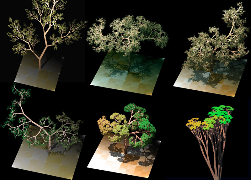
Graphical Interpretation
The graphical interpretation of L-systems transforms the derived strings into visual representations, typically using turtle graphics to simulate the growth of structures such as plants or fractals.[10][11] In this approach, the turtle maintains a state consisting of its current position, direction (heading angle), and pen status (whether it is drawing or moving without drawing).[11] The derived string from the L-system serves as a sequence of commands that guide the turtle's actions, enabling the depiction of branching patterns and recursive geometries.[10] To support drawing, the alphabet is augmented with symbols that control the turtle's movement and orientation. Common symbols include and , which instruct the turtle to move forward by a fixed step length while drawing a line for and without drawing for ; , which turns the turtle left by a specified angle ; and , which turns the turtle right by .[11] Branching is handled by , which pushes the current turtle state (position, heading, and pen status) onto a stack, and , which pops and restores the previous state, allowing substructures to emanate from a common point without altering the main path.[10] Other symbols from the original alphabet may be ignored during rendering or assigned additional interpretations as needed.[11] The rendering process involves sequentially traversing the derived string and executing each command in order. Starting from an initial position and heading, the turtle updates its state for each symbol: forward movements adjust the position based on the current heading, turns modify the heading angle, and stack operations manage branches recursively.[10] Key parameters include the step length , which defines the segment size; the turn angle , often set to values like 25.7° or 90° depending on the desired curvature; and scaling factors applied across iterations to prevent exponential growth in structure size, typically reducing by a factor such as (where is the golden ratio) for self-similar forms.[11] This method produces detailed 2D images that capture the iterative development of L-systems.[10] While primarily focused on 2D graphics, L-system rendering has been extended to 3D by incorporating additional axes and rotation commands, though these build on the same turtle principles without altering the core 2D interpretation.[11]Examples
Algae Growth
The classic example of an L-system modeling algal growth, introduced by Aristid Lindenmayer, uses a simple deterministic parallel rewriting mechanism to simulate the development of a linear filament of cells.[1] The axiom is the single symbol A, representing an initial cell.[1] The production rules are A → AB and B → A, where A denotes an active cell that divides into two cells (A and B), and B denotes an inactive cell that reverts to an active state in the next generation.[1] The derivation process begins with the axiom and applies the rules simultaneously to all symbols in each iteration. At iteration 0, the string is A. At iteration 1, it becomes AB. Iteration 2 yields ABA. By iteration 3, the string is ABAAB, and iteration 4 produces ABAABA. This sequence continues, with the length of the string at each step following the Fibonacci sequence (1, 2, 3, 5, 8, ...), reflecting the exponential growth pattern where each active cell contributes to proliferation.[1] In this model, the resulting string represents a one-dimensional chain of cells without branching, simulating synchronous cell division in a filament where cells alternate between active and inactive states to mimic division and maturation.[1] The system captures parallel development, as all cells evolve concurrently rather than sequentially. Biologically, it models the growth of unicellular strings in filamentous algae, such as Anabaena catenula, where cells form linear colonies through repeated division without lateral branching.[1] This L-system can be graphically interpreted using turtle graphics to render the filament as a straight line, with each symbol corresponding to a forward movement.Binary Fractal Tree
The binary fractal tree is a classic example of a graphical L-system that generates a self-similar branching structure resembling a tree through recursive application of production rules. This model uses a deterministic, context-free (D0L) L-system with bracketed symbols to simulate hierarchical branching, where each iteration expands the structure by adding symmetric left and right branches to existing segments. The system was popularized in computational plant modeling as a simple demonstration of how L-systems can produce fractal-like topologies that mimic natural dendritic growth patterns.[11] The axiom is F. The production rule is F → F[+F]F[-F]F, where F is a terminal symbol that remains unchanged. The angle of rotation is 45 degrees. In the turtle graphics interpretation, F instructs the turtle to move forward while drawing a line segment (representing a trunk or branch), + turns the turtle left by 45 degrees, - turns it right by 45 degrees, [ pushes the current position and orientation onto a stack to initiate a new branch, and ] pops the stack to resume from the saved state, enabling parallel branching. This setup ensures that branches are drawn without affecting the main stem, creating a binary hierarchy.[11] The derivation process unfolds iteratively through parallel rewriting, where all symbols in the current string are simultaneously replaced according to the rules. At iteration , the string is F, drawing a single line. At , the string becomes F[+F]F[-F]F, drawing a forward line (F), then a left branch ([+F]), a continuation (F), a right branch ([-F]), and final forward (F). By , it yields F[+F[+F]F[-F]F]F[-F[+F]F[-F]F]F, which adds sub-branches to the existing ones. At , the structure deepens further, forming a complete self-similar binary tree. Higher iterations increase the detail exponentially, with the number of F symbols (line segments) following the recurrence from the rules.[11] This L-system produces structures that approximate the topology of natural trees by recursively partitioning space into binary subdivisions, where branches fill the plane in a fractal manner, capturing the hierarchical and scale-invariant properties observed in real arboreal structures. The parallel rewriting inherent to L-systems aligns with simultaneous cellular growth in biology, enabling efficient simulation of developmental processes.[11]Cantor Set
The Cantor set, a canonical example of a fractal, can be generated using a deterministic L-system that models the iterative removal of middle-third intervals from the unit interval [0,1]. This approach captures the self-similar structure of the set through parallel string rewriting, where symbols represent preserved segments and removed gaps.[18] A standard L-system for the Cantor set uses the axiom and production rules , , with an alphabet consisting of non-terminals and and no constants. Here, symbolizes a preserved interval, while denotes a gap resulting from removal. An alternative variant employs rules , (the empty string), which explicitly simulates deletions by eliminating gap symbols in subsequent iterations. A graphical interpretation may map these to turtle graphics, where draws a line segment and advances without drawing, though the primary focus remains on the set-theoretic representation.[18][19] The derivation process mirrors the classical construction of the Cantor set. Starting with the axiom at iteration 0, which represents the full interval [0,1], the first application yields (iteration 1), dividing the interval into three equal parts and marking the middle as a gap. Iteration 2 produces , subdividing each preserved segment similarly and expanding gaps into three sub-gaps. Subsequent iterations continue this parallel rewriting, yielding a ternary structure where the limit string encodes the positions of remaining points: those with ternary expansions using only digits 0 and 2. This iterative middle-third removal results in preserved intervals of length at step , converging to a set of Lebesgue measure zero.[18][20] In set-theoretic terms, the final L-system string represents the Cantor set as the collection of intervals corresponding to symbols, with symbols indicating gaps. The self-similarity arises from the uniform scaling factor of and duplication of preserved parts, embodying the fractal's uncountably infinite yet measure-zero nature. L-systems thus provide a formal grammar for encoding this construction, facilitating analysis of its topological properties.[19] A key property demonstrated by this L-system is the Hausdorff dimension of the Cantor set, computed as , reflecting the scaling where two copies are produced at each third of the original size. This value, derived from the L-system's growth rates (two 's and three total subunits per iteration), underscores how such systems quantify fractal dimensions for self-similar structures.[20][21]Koch Curve
The Koch curve exemplifies the application of L-systems to generate fractal geometries, particularly through a deterministic rewriting process that produces a self-similar structure known as the Koch snowflake when closed.[8] In this L-system, the axiom is the string , representing an initial straight line segment.[8] The production rules are defined as , with constants remaining unchanged (, ), and the turtle interpretation uses an angle of 60° for turns.[8] Here, instructs the turtle to draw a forward segment, turns the turtle left by 60°, and turns it right by 60°, tracing the curve's boundary path.[8] The derivation process begins at iteration with the axiom , yielding a simple straight line.[8] At , the rule expands to , forming a bump-shaped protrusion on the line due to the turns.[8] Subsequent iterations apply the rule in parallel to each , recursively replacing segments and increasing complexity; as , the open curve approximates a closed snowflake boundary with infinite detail.[8] A key property is the exponential growth in curve length: each iteration multiplies the total length by , resulting in , where is the initial length, leading to an infinite perimeter for the snowflake while enclosing a finite area.[8] This contrast highlights the fractal's paradoxical nature, where the boundary becomes arbitrarily intricate without overlapping.[8] Parallel iteration of rules enables efficient computation of higher-order derivations despite exponential string growth.[8]Sierpinski Triangle
The Sierpinski triangle, a classic fractal also known as the Sierpinski gasket, can be approximated through an L-system that generates the Sierpinski arrowhead curve, a self-similar path whose limit traces the structure of the gasket via triangular subdivision. This L-system employs an alphabet with variables {A, B} and constants {+, −}, where the axiom is A. The production rules are A → +B−A−B+ and B → +A−B−A+, with a turn angle of 60° to align with the equilateral geometry of the triangle.[11] The derivation process begins with the axiom A and applies the rules in parallel to each variable iteratively, yielding strings that describe increasingly detailed paths. In the first iteration, A becomes +B−A−B+; the second iteration expands this to +(+A−B−A+)−(+B−A−B+)−(+A−B−A+)+, and further steps produce an arrowhead pattern—a zigzag motif that outlines the initial triangle and recursively subdivides it into smaller triangles, forming the gasket's characteristic voids. This iterative replacement doubles the string length each time while building the self-similar boundary.[10] Under turtle graphics interpretation, A and B both instruct drawing a forward line segment of fixed length, + denotes a left turn of 60°, and − a right turn of 60°. The rules' recursive structure ensures self-similarity, where each arrowhead segment spawns smaller copies oriented at 120° intervals, stacking to replicate the overall triangular form at every scale.[22] The resulting fractal exhibits a Hausdorff dimension of , quantifying its intermediate complexity between a line and a plane. Its Lebesgue measure (area) approaches 0, as the construction effectively removes half the area at the first step and one-quarter of the remaining at each subsequent iteration, converging to a set of measure zero. This L-system pattern also connects to cellular automata, where the Sierpinski triangle emerges in the evolution of Rule 90 under modulo-2 arithmetic, mirroring the same self-similar triangular voids.Dragon Curve
The dragon curve, a self-similar fractal curve, is generated using a deterministic L-system that models iterative paper-folding sequences, resulting in a twisting path reminiscent of a mythical dragon. The axiom is FX, with production rules X → X+YF+ and Y → −FX−Y, while F remains unchanged as a constant. The system employs a 90-degree angle for turns, where + denotes a left turn and − a right turn.[23] In graphical interpretation, the symbol F directs the turtle to move forward while drawing a line segment, whereas X and Y serve as non-drawing variables that recursively generate turns, enabling the system's fractal complexity without altering the drawing process directly. This interpretation simulates successive folds in a paper strip, where each iteration appends mirrored and rotated copies of the previous curve at right angles. The initial derivation at iteration n=0 yields FX, rendering a single straight line. Subsequent iterations apply the rules, doubling the string length each time and producing increasingly intricate twisting shapes that fold back on themselves. This L-system formulation is mathematically equivalent to an iterated function system defined by two affine transformations, each scaling by a factor of .[23][24] The resulting curve for finite iterations is non-self-intersecting in the plane, exhibiting self-overlapping in the sense that segments from later stages align closely with earlier ones without crossing, while maintaining overall self-similarity. In the infinite limit, it approaches a space-filling curve within a bounded region. The Hausdorff dimension of the curve's boundary is approximately 1.523.[24]Fractal Plant
The fractal plant L-system exemplifies the use of bracketed L-systems to model hierarchical branching structures in plants, incorporating elements like stems, branches, leaves, and buds to simulate realistic growth patterns.[11] Developed as part of early efforts in computational botany, this deterministic L-system begins with a simple axiom and applies parallel rewriting rules iteratively to generate a string that represents the plant's architecture.[11] The model emphasizes apical dominance, where the main stem suppresses lateral growth until later stages, leading to a central trunk with secondary branches and leaf attachments.[11] The axiom is defined asX, representing the initial apical meristem or growing tip of the plant.[11] The production rules are:
X → F[+X][-X]F[+XS][-XS]YS → S(whereSdenotes a leaf surface, often interpreted as a static leaf symbol without further rewriting)Y → (bud symbol, typically inert or terminal, representing a dormant bud)
F draws a stem segment, + and - indicate left and right turns, [ and ] push and pop the turtle's position and orientation to create branches, X is a non-drawing variable for further growth points, S attaches leaves, and Y marks potential future growth sites like buds.[11] The branch angle is set to 25.7°, while the divergence angle for leaf and bud placement approximates 137.5°, corresponding to the golden angle (approximately , where is the golden ratio) to achieve efficient spiral phyllotaxis that minimizes shading and maximizes light exposure.[11]
Iterations of the derivation process progressively build the plant's structure, starting from the axiom and applying the rules in parallel to all applicable symbols. For iteration 0 (n=0): X. At n=1: F[+X][-X]F[+XS][-XS]Y, which draws a short trunk (F), spawns two small branches ([+X][-X]), adds another stem segment (F), attaches leaves on additional branches ([+XS][-XS]), and ends with a bud (Y). By n=2, the string expands to include recursive branching on the main axis and laterals, forming a taller trunk with primary branches bearing secondary twigs and initial leaves (detailed transcription omitted for brevity; the structure follows parallel replacement of each X). Subsequent iterations (n=3 to 5) further subdivide branches, adding more leaves and buds, resulting in a bushy structure with a dominant vertical axis and spiraling laterals; at n=5, the model exhibits dense foliage while maintaining computational tractability for visualization.[11] Optional stochastic variations can introduce probabilistic rule selection (e.g., varying branch lengths or angles slightly) to simulate natural variability in plant specimens, though the base system remains deterministic.[11]
In graphical interpretation, a turtle graphics approach is employed, where the derived string is executed sequentially: F advances the turtle while drawing a line segment for stems, + and - rotate by the specified angles, and brackets [ and ] save and restore the turtle state to enable independent branch hierarchies without affecting the main stem.[11] The S symbol triggers rendering of leaf surfaces, often as polygons or textured primitives, while Y may halt drawing or place a bud marker. This setup mimics biological processes like apical dominance through the sequential placement of growth points, where the leading X continues the main axis longer than laterals, promoting upright growth.[11]
Biologically, the model's use of the golden angle ensures leaves and branches arrange in a spiral phyllotactic pattern, optimizing packing and sunlight capture as observed in many dicotyledonous plants; this addresses limitations in simpler fractal models by incorporating phyllotactic realism derived from Fibonacci-related divergence.[11] Such L-systems have influenced subsequent plant simulations by providing a foundation for integrating environmental interactions, though this example focuses on intrinsic developmental rules.[11]