


Community hub
Mandelbrot set
View on Wikipedia | This article needs additional citations for verification. (June 2024) |

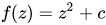
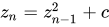
The Mandelbrot set (/ˈmændəlbroʊt, -brɒt/)[1][2] is a two-dimensional set that is defined in the complex plane as the complex numbers for which the function does not diverge to infinity when iterated starting at , i.e., for which the sequence , , etc., remains bounded in absolute value.[3]

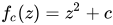


This set was first defined and drawn by Robert W. Brooks and Peter Matelski in 1978, as part of a study of Kleinian groups.[4] Afterwards, in 1980, Benoit Mandelbrot obtained high-quality visualizations of the set while working at IBM's Thomas J. Watson Research Center in Yorktown Heights, New York.[5]

Images of the Mandelbrot set exhibit an infinitely complicated boundary that reveals progressively ever-finer recursive detail at increasing magnifications;[6][7] mathematically, the boundary of the Mandelbrot set is a fractal curve.[8] The "style" of this recursive detail depends on the region of the set boundary being examined.[9] Mandelbrot set images may be created by sampling the complex numbers and testing, for each sample point , whether the sequence goes to infinity.[10][close paraphrasing] Treating the real and imaginary parts of as image coordinates on the complex plane, pixels may then be colored according to how soon the sequence crosses an arbitrarily chosen threshold (the threshold must be at least 2, as −2 is the complex number with the largest magnitude within the set, but otherwise the threshold is arbitrary).[10][close paraphrasing] If is held constant and the initial value of is varied instead, the corresponding Julia set for the point is obtained.[11]



The Mandelbrot set is well-known,[12] even outside mathematics,[13] for how it exhibits complex fractal structures when visualized and magnified, despite having a relatively simple definition, and is commonly cited as an example of mathematical beauty.[14][15][16]
History
[edit]
The Mandelbrot set has its origin in complex dynamics, a field first investigated by the French mathematicians Pierre Fatou and Gaston Julia at the beginning of the 20th century. The fractal was first defined and drawn in 1978 by Robert W. Brooks and Peter Matelski as part of a study of Kleinian groups.[4] On 1 March 1980, at IBM's Thomas J. Watson Research Center in Yorktown Heights, New York, Benoit Mandelbrot first visualized the set.[17]
Mandelbrot studied the parameter space of quadratic polynomials in an article that appeared in 1980.[18] The mathematical study of the Mandelbrot set really began with work by the mathematicians Adrien Douady and John H. Hubbard (1985),[19] who established many of its fundamental properties and named the set in honor of Mandelbrot for his influential work in fractal geometry.
The mathematicians Heinz-Otto Peitgen and Peter Richter became well known for promoting the set with photographs, books (1986),[20] and an internationally touring exhibit of the German Goethe-Institut (1985).[21][22]
The cover article of the August 1985 Scientific American introduced the algorithm for computing the Mandelbrot set. The cover was created by Peitgen, Richter and Saupe at the University of Bremen.[23] The Mandelbrot set became prominent in the mid-1980s as a computer-graphics demo, when personal computers became powerful enough to plot and display the set in high resolution.[24]
The work of Douady and Hubbard occurred during an increase in interest in complex dynamics and abstract mathematics,[25] and the topological and geometric study of the Mandelbrot set remains a key topic in the field of complex dynamics.[26]
Formal definition
[edit]
The Mandelbrot set is the uncountable set of values of c in the complex plane for which the orbit of the critical point under iteration of the quadratic map


remains bounded.[28] Thus, a complex number c is a member of the Mandelbrot set if, when starting with and applying the iteration repeatedly, the absolute value of remains bounded for all .


For example, for c = 1, the sequence is 0, 1, 2, 5, 26, ..., which tends to infinity, so 1 is not an element of the Mandelbrot set. On the other hand, for , the sequence is 0, −1, 0, −1, 0, ..., which is bounded, so −1 does belong to the set.

The Mandelbrot set can also be defined as the connectedness locus of the family of quadratic polynomials , the subset of the space of parameters for which the Julia set of the corresponding polynomial forms a connected set.[29] In the same way, the boundary of the Mandelbrot set can be defined as the bifurcation locus of this quadratic family, the subset of parameters near which the dynamic behavior of the polynomial (when it is iterated repeatedly) changes drastically.
Basic properties
[edit]The Mandelbrot set is a compact set, since it is closed and contained in the closed disk of radius 2 centred on zero. A point belongs to the Mandelbrot set if and only if for all . In other words, the absolute value of must remain at or below 2 for to be in the Mandelbrot set, , and if that absolute value exceeds 2, the sequence will escape to infinity. Since , it follows that , establishing that will always be in the closed disk of radius 2 around the origin.[30]


The intersection of with the real axis is the interval . The parameters along this interval can be put in one-to-one correspondence with those of the real logistic family,
![{\displaystyle \left[-2,{\frac {1}{4}}\right]}](https://wikimedia.org/api/rest_v1/media/math/render/svg/c22bf73a63f70e2801160f8680a43caad5ca10dd)
![{\displaystyle x_{n+1}=rx_{n}(1-x_{n}),\quad r\in [1,4].}](https://wikimedia.org/api/rest_v1/media/math/render/svg/167c3aa4bc1c5840ca0df792debf16643264a7f7)
The correspondence is given by

This gives a correspondence between the entire parameter space of the logistic family and that of the Mandelbrot set.[31]
Douady and Hubbard showed that the Mandelbrot set is connected. They constructed an explicit conformal isomorphism between the complement of the Mandelbrot set and the complement of the closed unit disk. Mandelbrot had originally conjectured that the Mandelbrot set is disconnected. This conjecture was based on computer pictures generated by programs that are unable to detect the thin filaments connecting different parts of . Upon further experiments, he revised his conjecture, deciding that should be connected. A topological proof of the connectedness was discovered in 2001 by Jeremy Kahn.[32]

The dynamical formula for the uniformisation of the complement of the Mandelbrot set, arising from Douady and Hubbard's proof of the connectedness of , gives rise to external rays of the Mandelbrot set. These rays can be used to study the Mandelbrot set in combinatorial terms and form the backbone of the Yoccoz parapuzzle.[33]
The boundary of the Mandelbrot set is the bifurcation locus of the family of quadratic polynomials. In other words, the boundary of the Mandelbrot set is the set of all parameters for which the dynamics of the quadratic map exhibits sensitive dependence on i.e. changes abruptly under arbitrarily small changes of It can be constructed as the limit set of a sequence of plane algebraic curves, the Mandelbrot curves, of the general type known as polynomial lemniscates. The Mandelbrot curves are defined by setting , and then interpreting the set of points in the complex plane as a curve in the real Cartesian plane of degree in x and y.[34] Each curve is the mapping of an initial circle of radius 2 under . These algebraic curves appear in images of the Mandelbrot set computed using the "escape time algorithm" mentioned below.





Other properties
[edit]Main cardioid and period bulbs
[edit]
The main cardioid is the period 1 continent.[35] It is the region of parameters for which the map has an attracting fixed point.[36] It consists of all parameters of the form for some in the open unit disk.[37][close paraphrasing]
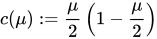

To the left of the main cardioid, attached to it at the point , a circular bulb, the period-2 bulb is visible.[37][close paraphrasing] The bulb consists of for which has an attracting cycle of period 2. It is the filled circle of radius 1/4 centered around −1.[37][close paraphrasing]


More generally, for every positive integer , there are circular bulbs tangent to the main cardioid called period-q bulbs (where denotes the Euler phi function), which consist of parameters for which has an attracting cycle of period .[citation needed] More specifically, for each primitive th root of unity (where ), there is one period-q bulb called the bulb, which is tangent to the main cardioid at the parameter and which contains parameters with -cycles having combinatorial rotation number .[38] More precisely, the periodic Fatou components containing the attracting cycle all touch at a common point (commonly called the -fixed point). If we label these components in counterclockwise orientation, then maps the component to the component .[37][close paraphrasing]






The change of behavior occurring at is known as a bifurcation: the attracting fixed point "collides" with a repelling period-q cycle. As we pass through the bifurcation parameter into the -bulb, the attracting fixed point turns into a repelling fixed point (the -fixed point), and the period-q cycle becomes attracting.[37][close paraphrasing]


Hyperbolic components
[edit]Bulbs that are interior components of the Mandelbrot set in which the maps have an attracting periodic cycle are called hyperbolic components.[39]
It is conjectured that these are the only interior regions of and that they are dense in . This problem, known as density of hyperbolicity, is one of the most important open problems in complex dynamics.[40] Hypothetical non-hyperbolic components of the Mandelbrot set are often referred to as "queer" or ghost components.[41][42] For real quadratic polynomials, this question was proved in the 1990s independently by Lyubich and by Graczyk and Świątek. (Note that hyperbolic components intersecting the real axis correspond exactly to periodic windows in the Feigenbaum diagram. So this result states that such windows exist near every parameter in the diagram.)
Not every hyperbolic component can be reached by a sequence of direct bifurcations from the main cardioid of the Mandelbrot set. Such a component can be reached by a sequence of direct bifurcations from the main cardioid of a little Mandelbrot copy (see below).

Each of the hyperbolic components has a center, which is a point c such that the inner Fatou domain for has a super-attracting cycle—that is, that the attraction is infinite. This means that the cycle contains the critical point 0, so that 0 is iterated back to itself after some iterations. Therefore, for some n. If we call this polynomial (letting it depend on c instead of z), we have that and that the degree of is . Therefore, constructing the centers of the hyperbolic components is possible by successively solving the equations .[citation needed] The number of new centers produced in each step is given by Sloane's (sequence A000740 in the OEIS).





Local connectivity
[edit]It is conjectured that the Mandelbrot set is locally connected. This conjecture is known as MLC (for Mandelbrot locally connected). By the work of Adrien Douady and John H. Hubbard, this conjecture would result in a simple abstract "pinched disk" model of the Mandelbrot set. In particular, it would imply the important hyperbolicity conjecture mentioned above.[citation needed]
The work of Jean-Christophe Yoccoz established local connectivity of the Mandelbrot set at all finitely renormalizable parameters; that is, roughly speaking those contained only in finitely many small Mandelbrot copies.[43] Since then, local connectivity has been proved at many other points of , but the full conjecture is still open.
Self-similarity
[edit]
The Mandelbrot set is self-similar under magnification in the neighborhoods of the Misiurewicz points. It is also conjectured to be self-similar around generalized Feigenbaum points (e.g., −1.401155 or −0.1528 + 1.0397i), in the sense of converging to a limit set.[44][45] The Mandelbrot set in general is quasi-self-similar, as small slightly different versions of itself can be found at arbitrarily small scales. These copies of the Mandelbrot set are all slightly different, mostly because of the thin threads connecting them to the main body of the set.[46]
Further results
[edit]The Hausdorff dimension of the boundary of the Mandelbrot set equals 2 as determined by a result of Mitsuhiro Shishikura.[47] The fact that this is greater by a whole integer than its topological dimension, which is 1, reflects the extreme fractal nature of the Mandelbrot set boundary. Roughly speaking, Shishikura's result states that the Mandelbrot set boundary is so "wiggly" that it locally fills space as efficiently as a two-dimensional planar region. Curves with Hausdorff dimension 2, despite being (topologically) 1-dimensional, are oftentimes capable of having nonzero area (more formally, a nonzero planar Lebesgue measure). Whether this is the case for the Mandelbrot set boundary is an unsolved problem.[citation needed]
It has been shown that the generalized Mandelbrot set in higher-dimensional hypercomplex number spaces (i.e. when the power of the iterated variable tends to infinity) is convergent to the unit (−1)-sphere.[48]
In the Blum–Shub–Smale model of real computation, the Mandelbrot set is not computable, but its complement is computably enumerable. Many simple objects (e.g., the graph of exponentiation) are also not computable in the BSS model. At present, it is unknown whether the Mandelbrot set is computable in models of real computation based on computable analysis, which correspond more closely to the intuitive notion of "plotting the set by a computer". Hertling has shown that the Mandelbrot set is computable in this model if the hyperbolicity conjecture is true.[citation needed]
Relationship with Julia sets
[edit]
As a consequence of the definition of the Mandelbrot set, there is a close correspondence between the geometry of the Mandelbrot set at a given point and the structure of the corresponding Julia set. For instance, a value of c belongs to the Mandelbrot set if and only if the corresponding Julia set is connected. Thus, the Mandelbrot set may be seen as a map of the connected Julia sets.[49][better source needed]
This principle is exploited in virtually all deep results on the Mandelbrot set. For example, Shishikura proved that, for a dense set of parameters in the boundary of the Mandelbrot set, the Julia set has Hausdorff dimension two, and then transfers this information to the parameter plane.[47] Similarly, Yoccoz first proved the local connectivity of Julia sets, before establishing it for the Mandelbrot set at the corresponding parameters.[43]
Geometry
[edit]For every rational number , where p and q are coprime, a hyperbolic component of period q bifurcates from the main cardioid at a point on the edge of the cardioid corresponding to an internal angle of .[50] The part of the Mandelbrot set connected to the main cardioid at this bifurcation point is called the p/q-limb. Computer experiments suggest that the diameter of the limb tends to zero like . The best current estimate known is the Yoccoz-inequality, which states that the size tends to zero like .[citation needed]


A period-q limb will have "antennae" at the top of its limb. The period of a given bulb is determined by counting these antennas. The numerator of the rotation number, p, is found by numbering each antenna counterclockwise from the limb from 1 to and finding which antenna is the shortest.[50]

Pi in the Mandelbrot set
[edit]There are intriguing experiments in the Mandelbrot set that lead to the occurrence of the number . For a parameter with , verifying that is not in the Mandelbrot set means iterating the sequence starting with , until the sequence leaves the disk around of any radius . This is motivated by the (still open) question whether the vertical line at real part intersects the Mandelbrot set at points away from the real line. It turns out that the necessary number of iterations, multiplied by , converges to pi. For example, for = 0.0000001, and , the number of iterations is 31415928 and the product is 3.1415928.[51] This experiment was performed independently by many people in the early 1990s, if not before; for instance by David Boll.


Analogous observations have also been made at the parameters and (with a necessary modification in the latter case). In 2001, Aaron Klebanoff published a (non-conceptual) proof for this phenomenon at [52]


In 2023, Paul Siewert developed, in his Bachelor thesis, a conceptual proof also for the value , explaining why the number pi occurs (geometrically as half the circumference of the unit circle).[53]
In 2025, the three high school students Thies Brockmöller, Oscar Scherz, and Nedim Srkalovic extended the theory and the conceptual proof to all the infinitely bifurcation points in the Mandelbrot set.[54]
Fibonacci sequence in the Mandelbrot set
[edit]The Mandelbrot Set features a fundamental cardioid shape adorned with numerous bulbs directly attached to it.[55] Understanding the arrangement of these bulbs requires a detailed examination of the Mandelbrot Set's boundary. As one zooms into specific portions with a geometric perspective, precise deducible information about the location within the boundary and the corresponding dynamical behavior for parameters drawn from associated bulbs emerges.[56]
The iteration of the quadratic polynomial , where is a parameter drawn from one of the bulbs attached to the main cardioid within the Mandelbrot Set, gives rise to maps featuring attracting cycles of a specified period and a rotation number . In this context, the attracting cycle of exhibits rotational motion around a central fixed point, completing an average of revolutions at each iteration.[56][57]

The bulbs within the Mandelbrot Set are distinguishable by both their attracting cycles and the geometric features of their structure. Each bulb is characterized by an antenna attached to it, emanating from a junction point and displaying a certain number of spokes indicative of its period. For instance, the bulb is identified by its attracting cycle with a rotation number of . Its distinctive antenna-like structure comprises a junction point from which five spokes emanate. Among these spokes, called the principal spoke is directly attached to the bulb, and the 'smallest' non-principal spoke is positioned approximately of a turn counterclockwise from the principal spoke, providing a distinctive identification as a -bulb.[58] This raises the question: how does one discern which among these spokes is the 'smallest'?[55][58] In the theory of external rays developed by Douady and Hubbard,[59] there are precisely two external rays landing at the root point of a satellite hyperbolic component of the Mandelbrot Set. Each of these rays possesses an external angle that undergoes doubling under the angle doubling map . According to this theorem, when two rays land at the same point, no other rays between them can intersect. Thus, the 'size' of this region is measured by determining the length of the arc between the two angles.[56]


If the root point of the main cardioid is the cusp at , then the main cardioid is the -bulb. The root point of any other bulb is just the point where this bulb is attached to the main cardioid. This prompts the inquiry: which is the largest bulb between the root points of the and -bulbs? It is clearly the -bulb. And note that is obtained from the previous two fractions by Farey addition, i.e., adding the numerators and adding the denominators


Similarly, the largest bulb between the and -bulbs is the -bulb, again given by Farey addition.

The largest bulb between the and -bulb is the -bulb, while the largest bulb between the and -bulbs is the -bulb, and so on.[56][60] The arrangement of bulbs within the Mandelbrot set follows a remarkable pattern governed by the Farey tree, a structure encompassing all rationals between and . This ordering positions the bulbs along the boundary of the main cardioid precisely according to the rational numbers in the unit interval.[58]


Starting with the bulb at the top and progressing towards the circle, the sequence unfolds systematically: the largest bulb between and is , between and is , and so forth.[61] Intriguingly, the denominators of the periods of circular bulbs at sequential scales in the Mandelbrot Set conform to the Fibonacci number sequence, the sequence that is made by adding the previous two terms – 1, 2, 3, 5, 8, 13, 21...[62][63]
The Fibonacci sequence manifests in the number of spiral arms at a unique spot on the Mandelbrot set, mirrored both at the top and bottom. This distinctive location demands the highest number of iterations of for a detailed fractal visual, with intricate details repeating as one zooms in.[64]
Image gallery of a zoom sequence
[edit]The boundary of the Mandelbrot set shows more intricate detail the closer one looks or magnifies the image. The following is an example of an image sequence zooming to a selected c value. The area shown is known as the "seahorse valley", which is a region of the Mandelbrot set centred on the point −0.75 + 0.1i.[65]
The magnification of the last image relative to the first one is about 1010 to 1. Relating to an ordinary computer monitor, it represents a section of a Mandelbrot set with a diameter of 4 million kilometers.
-
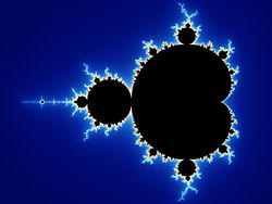 Start. Mandelbrot set with continuously colored environment.
 -
![Gap between the "head" and the "body", also called the "seahorse valley"[66]](//upload.wikimedia.org/wikipedia/commons/thumb/e/ee/Mandel_zoom_01_head_and_shoulder.jpg/250px-Mandel_zoom_01_head_and_shoulder.jpg) Gap between the "head" and the "body", also called the "seahorse valley"[66]
Gap between the "head" and the "body", also called the "seahorse valley"[66] -
 Double-spirals on the left, "seahorses" on the right
 -
 "Seahorse" upside down
![Gap between the "head" and the "body", also called the "seahorse valley"[66]](https://en.wikipedia.org/wiki/File:Mandel_zoom_01_head_and_shoulder.jpg)


The seahorse "body" is composed by 25 "spokes" consisting of two groups of 12 "spokes"[67] each and one "spoke" connecting to the main cardioid. These two groups can be attributed by some metamorphosis to the two "fingers" of the "upper hand" of the Mandelbrot set; therefore, the number of "spokes" increases from one "seahorse" to the next by 2; the "hub" is a Misiurewicz point. Between the "upper part of the body" and the "tail", there is a distorted copy of the Mandelbrot set, called a "satellite".
-
 The central endpoint of the "seahorse tail" is also a Misiurewicz point.
 -
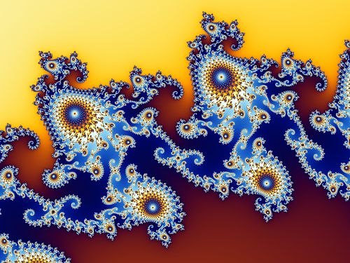 Part of the "tail" – there is only one path consisting of the thin structures that lead through the whole "tail". This zigzag path passes the "hubs" of the large objects with 25 "spokes" at the inner and outer border of the "tail"; thus the Mandelbrot set is a simply connected set, which means there are no islands and no loop roads around a hole.
 -
![Satellite. The two "seahorse tails" (also called dendritic structures)[68] are the beginning of a series of concentric crowns with the satellite in the center.](//upload.wikimedia.org/wikipedia/commons/thumb/f/f3/Mandel_zoom_06_double_hook.jpg/500px-Mandel_zoom_06_double_hook.jpg) Satellite. The two "seahorse tails" (also called dendritic structures)[68] are the beginning of a series of concentric crowns with the satellite in the center.
Satellite. The two "seahorse tails" (also called dendritic structures)[68] are the beginning of a series of concentric crowns with the satellite in the center. -
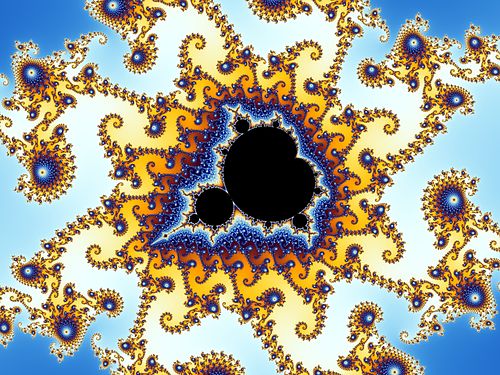 Each of these crowns consists of similar "seahorse tails"; their number increases with powers of 2, a typical phenomenon in the environment of satellites. The unique path to the spiral center passes the satellite from the groove of the cardioid to the top of the "antenna" on the "head".
 -
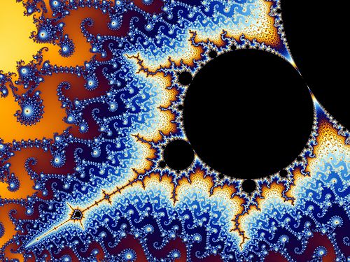 "Antenna" of the satellite. There are several satellites of second order.
 -
![The "seahorse valley"[66] of the satellite. All the structures from the start reappear.](//upload.wikimedia.org/wikipedia/commons/thumb/2/2f/Mandel_zoom_09_satellite_head_and_shoulder.jpg/500px-Mandel_zoom_09_satellite_head_and_shoulder.jpg) The "seahorse valley"[66] of the satellite. All the structures from the start reappear.
The "seahorse valley"[66] of the satellite. All the structures from the start reappear. -
 Double-spirals and "seahorses" – unlike the second image from the start, they have appendices consisting of structures like "seahorse tails"; this demonstrates the typical linking of n + 1 different structures in the environment of satellites of the order n, here for the simplest case n = 1.
 -
 Double-spirals with satellites of second order – analogously to the "seahorses", the double-spirals may be interpreted as a metamorphosis of the "antenna".
 -
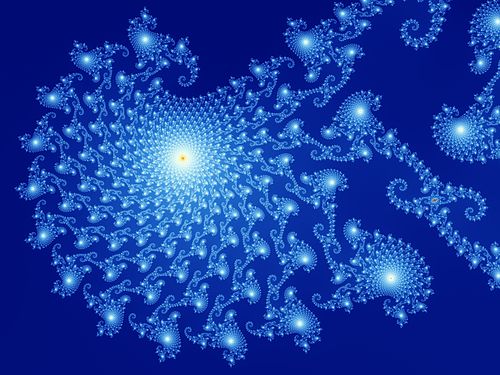 In the outer part of the appendices, islands of structures may be recognized; they have a shape like Julia sets Jc; the largest of them may be found in the center of the "double-hook" on the right side.
 -
 Part of the "double-hook".
 -
 Islands.
 -
 A detail of one island.
 -
 Detail of the spiral.


![Satellite. The two "seahorse tails" (also called dendritic structures)[68] are the beginning of a series of concentric crowns with the satellite in the center.](https://en.wikipedia.org/wiki/File:Mandel_zoom_06_double_hook.jpg)


![The "seahorse valley"[66] of the satellite. All the structures from the start reappear.](https://en.wikipedia.org/wiki/File:Mandel_zoom_09_satellite_head_and_shoulder.jpg)


The islands in the third-to-last step seem to consist of infinitely many parts, as is the case for the corresponding Julia set . They are connected by tiny structures, so that the whole represents a simply connected set. The tiny structures meet each other at a satellite in the center that is too small to be recognized at this magnification. The value of for the corresponding is not the image center but, relative to the main body of the Mandelbrot set, has the same position as the center of this image relative to the satellite shown in the 6th step.

Inner structure
[edit]While the Mandelbrot set is typically rendered showing outside boundary detail, structure within the bounded set can also be revealed.[69][70][71] For example, while calculating whether or not a given c value is bound or unbound, while it remains bound, the maximum value that this number reaches can be compared to the c value at that location. If the sum of squares method is used, the calculated number would be max:(real^2 + imaginary^2) − c:(real^2 + imaginary^2).[citation needed] The magnitude of this calculation can be rendered as a value on a gradient.
This produces results like the following, gradients with distinct edges and contours as the boundaries are approached. The animations serve to highlight the gradient boundaries.
-
 Animated gradient structure inside the Mandelbrot set
 -
 Animated gradient structure inside the Mandelbrot set, detail
 -
 Rendering of progressive iterations from 285 to approximately 200,000 with corresponding bounded gradients animated
 -
 Thumbnail for gradient in progressive iterations


Generalizations
[edit]

Multibrot sets
[edit]Multibrot sets are bounded sets found in the complex plane for members of the general monic univariate polynomial family of recursions
- .[72]

For an integer d, these sets are connectedness loci for the Julia sets built from the same formula. The full cubic connectedness locus has also been studied; here one considers the two-parameter recursion , whose two critical points are the complex square roots of the parameter k. A parameter is in the cubic connectedness locus if both critical points are stable.[73] For general families of holomorphic functions, the boundary of the Mandelbrot set generalizes to the bifurcation locus.[citation needed]

The Multibrot set is obtained by varying the value of the exponent d. The article has a video that shows the development from d = 0 to 7, at which point there are 6 i.e. lobes around the perimeter. In general, when d is a positive integer, the central region in each of these sets is always an epicycloid of cusps. A similar development with negative integral exponents results in clefts on the inside of a ring, where the main central region of the set is a hypocycloid of cusps.[citation needed]


Higher dimensions
[edit]There is no perfect extension of the Mandelbrot set into 3D, because there is no 3D analogue of the complex numbers for it to iterate on. There is an extension of the complex numbers into 4 dimensions, the quaternions, that creates a perfect extension of the Mandelbrot set and the Julia sets into 4 dimensions.[74] These can then be either cross-sectioned or projected into a 3D structure. The quaternion (4-dimensional) Mandelbrot set is simply a solid of revolution of the 2-dimensional Mandelbrot set (in the j-k plane), and is therefore uninteresting to look at.[74] Taking a 3-dimensional cross section at results in a solid of revolution of the 2-dimensional Mandelbrot set around the real axis.[citation needed]

Other non-analytic mappings
[edit]
The tricorn fractal, also called the Mandelbar set, is the connectedness locus of the anti-holomorphic family .[75][76] It was encountered by Milnor in his study of parameter slices of real cubic polynomials.[citation needed] It is not locally connected.[75] This property is inherited by the connectedness locus of real cubic polynomials.[citation needed]

Another non-analytic generalization is the Burning Ship fractal, which is obtained by iterating the following:

Computer drawings
[edit]There exist a multitude of various algorithms for plotting the Mandelbrot set via a computing device. Here, the naïve[77] "escape time algorithm" will be shown, since it is the most popular[78] and one of the simplest algorithms.[79] In the escape time algorithm, a repeating calculation is performed for each x, y point in the plot area and based on the behavior of that calculation, a color is chosen for that pixel.[80][81]
The x and y locations of each point are used as starting values in a repeating, or iterating calculation (described in detail below). The result of each iteration is used as the starting values for the next. The values are checked during each iteration to see whether they have reached a critical "escape" condition, or "bailout". If that condition is reached, the calculation is stopped, the pixel is drawn, and the next x, y point is examined.
The color of each point represents how quickly the values reached the escape point. Often black is used to show values that fail to escape before the iteration limit, and gradually brighter colors are used for points that escape. This gives a visual representation of how many cycles were required before reaching the escape condition.
To render such an image, the region of the complex plane we are considering is subdivided into a certain number of pixels. To color any such pixel, let be the midpoint of that pixel. Iterate the critical point 0 under , checking at each step whether the orbit point has a radius larger than 2. When this is the case, does not belong to the Mandelbrot set, and color the pixel according to the number of iterations used to find out. Otherwise, keep iterating up to a fixed number of steps, after which we decide that our parameter is "probably" in the Mandelbrot set, or at least very close to it, and color the pixel black.
In pseudocode, this algorithm would look as follows. The algorithm does not use complex numbers and manually simulates complex-number operations using two real numbers, for those who do not have a complex data type. The program may be simplified if the programming language includes complex-data-type operations.
for each pixel (Px, Py) on the screen do
    x0 := scaled x coordinate of pixel (scaled to lie in the Mandelbrot X scale (-2.00, 0.47))
    y0 := scaled y coordinate of pixel (scaled to lie in the Mandelbrot Y scale (-1.12, 1.12))
    x := 0.0
    y := 0.0
    iteration := 0
    max_iteration := 1000
    while (x^2 + y^2 ≤ 2^2 AND iteration < max_iteration) do
        xtemp := x^2 - y^2 + x0
        y := 2*x*y + y0
        x := xtemp
        iteration := iteration + 1

    color := palette[iteration]
    plot(Px, Py, color)
Here, relating the pseudocode to , and :


and so, as can be seen in the pseudocode in the computation of x and y:
- and .


To get colorful images of the set, the assignment of a color to each value of the number of executed iterations can be made using one of a variety of functions (linear, exponential, etc.).
Python code
[edit]Here is the code implementing the above algorithm in Python:[82][close paraphrasing]
import numpy as np
import matplotlib.pyplot as plt

# Setting parameters (these values can be changed)
x_domain, y_domain = np.linspace(-2, 2, 500), np.linspace(-2, 2, 500)
bound = 2
max_iterations = 50  # any positive integer value
colormap = "nipy_spectral"  # set to any matplotlib valid colormap

func = lambda z, p, c: z**p + c

# Computing 2D array to represent the Mandelbrot set
iteration_array = []
for y in y_domain:
    row = []
    for x in x_domain:
        z = 0
        p = 2
        c = complex(x, y)
        for iteration_number in range(max_iterations):
            if abs(z) >= bound:
                row.append(iteration_number)
                break
            else:
                try:
                    z = func(z, p, c)
                except (ValueError, ZeroDivisionError):
                    z = c
        else:
            row.append(0)

    iteration_array.append(row)

# Plotting the data
ax = plt.axes()
ax.set_aspect("equal")
graph = ax.pcolormesh(x_domain, y_domain, iteration_array, cmap=colormap)
plt.colorbar(graph)
plt.xlabel("Real-Axis")
plt.ylabel("Imaginary-Axis")
plt.show()


The value of power variable can be modified to generate an image of equivalent multibrot set (). For example, setting p = 2 produces the associated image.

References in popular culture
[edit]The Mandelbrot set is widely considered the most popular fractal,[83][84] and has been referenced several times in popular culture.
Comics & Manga
[edit]- The unfinished Alan Moore comic book series Big Numbers (1990) used Mandelbrot's work on fractal geometry and chaos theory to underpin the structure of that work. Moore at one point was going to name the comic book series The Mandelbrot Set.[85]
- In the manga The Summer Hikaru Died (2021 – present), Yoshiki hallucinates the Mandelbrot set when he reaches into the body of the false Hikaru.
Literature
[edit]- The Arthur C. Clarke novel The Ghost from the Grand Banks (1990) features an artificial lake made to replicate the shape of the Mandelbrot set.[86]
- The second book of the Mode series by Piers Anthony, Fractal Mode (1992), describes a world that is a perfect 3D model of the set.[87]
- In Ian Stewart's 2001 book Flatterland, there is a character called the Mandelblot, who helps explain fractals to the characters and reader.[88]
Music
[edit]- Blue Man Group's 1999 debut album Audio references the Mandelbrot set in the titles of the songs "Opening Mandelbrot", "Mandelgroove", and "Klein Mandelbrot".[89] Their second album, The Complex (2003), closes with a hidden track titled "Mandelbrot IV".
- The American rock band Heart has an image of a Mandelbrot set on the cover of their album Jupiters Darling (2004).
- The British black metal band Anaal Nathrakh uses an image resembling the Mandelbrot set on their Eschaton (2006) album cover art.
- The Jonathan Coulton song "Mandelbrot Set" (2008) is a tribute to both the fractal itself and to the man it is named after, Benoit Mandelbrot.[90]
- The Neil Cicierega song "It's Gonna Get Weird" (2016) is an unused song written for Gravity Falls (2012 – 2016) sung from the perspective of main antagonist Bill Cipher.[91][92] In one verse, Bill considers creating "Mandelbrot rainbows" and "screaming tornadoes".[93]
Other
[edit]- The television series Dirk Gently's Holistic Detective Agency (2016) prominently features the Mandelbrot set in connection with the visions of the character Amanda. In the second season, her jacket has a large image of the fractal on the back.[94]
- Benoit Mandelbrot and the eponymous set were the subjects of the Google Doodle on 20 November 2020 (the late Benoit Mandelbrot's 96th birthday).[95]
See also
[edit]References
[edit]- ^ "Mandelbrot set". Lexico UK English Dictionary. Oxford University Press. Archived from the original on 31 January 2022.
- ^ "Mandelbrot set". Merriam-Webster.com Dictionary. Merriam-Webster. Retrieved 30 January 2022.
- ^ Cooper, S. B.; Löwe, Benedikt; Sorbi, Andrea (28 November 2007). New Computational Paradigms: Changing Conceptions of What is Computable. Springer Science & Business Media. p. 450. ISBN 978-0-387-68546-5.
- ^ a b Robert Brooks and Peter Matelski, The dynamics of 2-generator subgroups of PSL(2,C), in Irwin Kra (1981). Irwin Kra (ed.). Riemann Surfaces and Related Topics: Proceedings of the 1978 Stony Brook Conference (PDF). Bernard Maskit. Princeton University Press. ISBN 0-691-08267-7. Archived from the original (PDF) on 28 July 2019. Retrieved 1 July 2019.
- ^ Nakos, George (20 May 2024). Elementary Linear Algebra with Applications: MATLAB®, Mathematica® and MaplesoftTM. Walter de Gruyter GmbH & Co KG. p. 322. ISBN 978-3-11-133185-0.
- ^ Addison, Paul S. (1 January 1997). Fractals and Chaos: An illustrated course. CRC Press. p. 110. ISBN 978-0-8493-8443-1.
- ^ Briggs, John (1992). Fractals: The Patterns of Chaos : a New Aesthetic of Art, Science, and Nature. Simon and Schuster. p. 77. ISBN 978-0-671-74217-1.
- ^ Hewson, Stephen Fletcher (2009). A Mathematical Bridge: An Intuitive Journey in Higher Mathematics. World Scientific. p. 155. ISBN 978-981-283-407-2.
- ^ Peitgen, Heinz-Otto; Richter, Peter H. (1 December 2013). The Beauty of Fractals: Images of Complex Dynamical Systems. Springer Science & Business Media. p. 166. ISBN 978-3-642-61717-1.
the Mandelbrot set is very diverse in its different regions
- ^ a b Hunt, John (1 October 2023). Advanced Guide to Python 3 Programming. Springer Nature. p. 117. ISBN 978-3-031-40336-1.
- ^ Campuzano, Juan Carlos Ponce (20 November 2020). "Complex Analysis". Complex Analysis — The Mandelbrot Set. Archived from the original on 16 October 2024. Retrieved 5 March 2025.
- ^ Oberguggenberger, Michael; Ostermann, Alexander (24 October 2018). Analysis for Computer Scientists: Foundations, Methods, and Algorithms. Springer. p. 131. ISBN 978-3-319-91155-7.
- ^ "Mandelbrot Set". cometcloud.sci.utah.edu. Retrieved 22 March 2025.
- ^ Peitgen, Heinz-Otto; Jürgens, Hartmut; Saupe, Dietmar (6 December 2012). Fractals for the Classroom: Part Two: Complex Systems and Mandelbrot Set. Springer Science & Business Media. p. 415. ISBN 978-1-4612-4406-6.
- ^ Gulick, Denny; Ford, Jeff (10 May 2024). Encounters with Chaos and Fractals. CRC Press. pp. §7.2. ISBN 978-1-003-83578-3.
- ^ Bialynicki-Birula, Iwo; Bialynicka-Birula, Iwona (21 October 2004). Modeling Reality: How Computers Mirror Life. OUP Oxford. p. 80. ISBN 978-0-19-853100-5.
- ^ R.P. Taylor & J.C. Sprott (2008). "Biophilic Fractals and the Visual Journey of Organic Screen-savers" (PDF). Nonlinear Dynamics, Psychology, and Life Sciences. 12 (1). Society for Chaos Theory in Psychology & Life Sciences: 117–129. PMID 18157930. Retrieved 1 January 2009.
- ^ Mandelbrot, Benoit (1980). "Fractal aspects of the iteration of for complex ". Annals of the New York Academy of Sciences. 357 (1): 249–259. doi:10.1111/j.1749-6632.1980.tb29690.x. S2CID 85237669.
- ^ Adrien Douady and John H. Hubbard, Etude dynamique des polynômes complexes, Prépublications mathémathiques d'Orsay 2/4 (1984 / 1985)
- ^ Peitgen, Heinz-Otto; Richter Peter (1986). The Beauty of Fractals. Heidelberg: Springer-Verlag. ISBN 0-387-15851-0.
- ^ Frontiers of Chaos, Exhibition of the Goethe-Institut by H.O. Peitgen, P. Richter, H. Jürgens, M. Prüfer, D.Saupe. Since 1985 shown in over 40 countries.
- ^ Gleick, James (1987). Chaos: Making a New Science. London: Cardinal. p. 229.
- ^ "Exploring The Mandelbrot Set". Scientific American. 253 (2): 4. August 1985. JSTOR 24967754.
- ^ Pountain, Dick (September 1986). "Turbocharging Mandelbrot". Byte. Retrieved 11 November 2015.
- ^ Rees, Mary (January 2016). "One hundred years of complex dynamics". Proceedings of the Royal Society A: Mathematical, Physical and Engineering Sciences. 472 (2185). Bibcode:2016RSPSA.47250453R. doi:10.1098/rspa.2015.0453. PMC 4786033. PMID 26997888.
- ^ Schleicher, Dierk (3 November 2009). Complex Dynamics: Families and Friends. CRC Press. pp. xii. ISBN 978-1-4398-6542-2.
- ^ Weisstein, Eric W. "Mandelbrot Set". mathworld.wolfram.com. Retrieved 24 January 2024.
- ^ "Mandelbrot Set Explorer: Mathematical Glossary". Retrieved 7 October 2007.
- ^ Tiozzo, Giulio (15 May 2013), Topological entropy of quadratic polynomials and dimension of sections of the Mandelbrot set, arXiv:1305.3542
- ^ "Escape Radius". Retrieved 17 January 2024.
- ^ thatsmaths (7 December 2023). "The Logistic Map is hiding in the Mandelbrot Set". ThatsMaths. Retrieved 18 February 2024.
- ^ Kahn, Jeremy (8 August 2001). "The Mandelbrot Set is Connected: a Topological Proof" (PDF).
- ^ The Mandelbrot set, theme and variations. Tan, Lei. Cambridge University Press, 2000. ISBN 978-0-521-77476-5. Section 2.1, "Yoccoz para-puzzles", p. 121
- ^ Weisstein, Eric W. "Mandelbrot Set Lemniscate". Wolfram Mathworld. Retrieved 17 July 2023.
- ^ Brucks, Karen M.; Bruin, Henk (28 June 2004). Topics from One-Dimensional Dynamics. Cambridge University Press. p. 264. ISBN 978-0-521-54766-6.
- ^ Devaney, Robert (9 March 2018). An Introduction To Chaotic Dynamical Systems. CRC Press. p. 147. ISBN 978-0-429-97085-6.
- ^ a b c d e Ivancevic, Vladimir G.; Ivancevic, Tijana T. (6 February 2007). High-Dimensional Chaotic and Attractor Systems: A Comprehensive Introduction. Springer Science & Business Media. pp. 492–493. ISBN 978-1-4020-5456-3.
- ^ Devaney, Robert L.; Branner, Bodil (1994). Complex Dynamical Systems: The Mathematics Behind the Mandelbrot and Julia Sets: The Mathematics Behind the Mandelbrot and Julia Sets. American Mathematical Soc. pp. 18–19. ISBN 978-0-8218-0290-8.
- ^ Redona, Jeffrey Francis (1996). The Mandelbrot set (Masters of Arts in Mathematics). Theses Digitization Project.
- ^ Anna Miriam Benini (2017). "A survey on MLC, Rigidity and related topics". arXiv:1709.09869 [math.DS].
- ^ Douady, Adrien; Hubbard, John H. Exploring the Mandelbrot set. The Orsay Notes. p. 12.
- ^ Jung, Wolf (2002). Homeomorphisms on Edges of the Mandelbrot Set (Doctoral thesis). RWTH Aachen University. urn:nbn:de:hbz:82-opus-3719.
- ^ a b Hubbard, J. H. (1993). "Local connectivity of Julia sets and bifurcation loci: three theorems of J.-C. Yoccoz" (PDF). Topological methods in modern mathematics (Stony Brook, NY, 1991). Houston, TX: Publish or Perish. pp. 467–511. MR 1215974.. Hubbard cites as his source a 1989 unpublished manuscript of Yoccoz.
- ^ Lei (1990). "Similarity between the Mandelbrot set and Julia Sets". Communications in Mathematical Physics. 134 (3): 587–617. Bibcode:1990CMaPh.134..587L. doi:10.1007/bf02098448. S2CID 122439436.
- ^ J. Milnor (1989). "Self-Similarity and Hairiness in the Mandelbrot Set". In M. C. Tangora (ed.). Computers in Geometry and Topology. New York: Taylor & Francis. pp. 211–257. ISBN 9780824780319.)
- ^ "Mandelbrot Viewer". math.hws.edu. Retrieved 1 March 2025.
- ^ a b Shishikura, Mitsuhiro (1998). "The Hausdorff dimension of the boundary of the Mandelbrot set and Julia sets". Annals of Mathematics. Second Series. 147 (2): 225–267. arXiv:math.DS/9201282. doi:10.2307/121009. JSTOR 121009. MR 1626737. S2CID 14847943..
- ^ Katunin, Andrzej; Fedio, Kamil (2015). "On a Visualization of the Convergence of the Boundary of Generalized Mandelbrot Set to (n-1)-Sphere" (PDF). Journal of Applied Mathematics and Computational Mechanics. 14 (1): 63–69. doi:10.17512/jamcm.2015.1.06. Retrieved 18 May 2022.
- ^ Sims, Karl. "Understanding Julia and Mandelbrot Sets". karlsims.com. Retrieved 27 January 2025.
- ^ a b "Number Sequences in the Mandelbrot Set". youtube.com. The Mathemagicians' Guild. 4 June 2020. Archived from the original on 30 October 2021.
- ^ Flake, Gary William (1998). The Computational Beauty of Nature. MIT Press. p. 125. ISBN 978-0-262-56127-3.
- ^ Klebanoff, Aaron D. (2001). "π in the Mandelbrot Set". Fractals. 9 (4): 393–402. doi:10.1142/S0218348X01000828.
- ^ Paul Siewert, Pi in the Mandelbrot set. Bachelor Thesis, Universität Göttingen, 2023
- ^ Brockmoeller, Thies; Scherz, Oscar; Srkalovic, Nedim (2025). "Pi in the Mandelbrot set everywhere". arXiv:2505.07138 [math.DS].
- ^ a b Devaney, Robert L. (April 1999). "The Mandelbrot Set, the Farey Tree, and the Fibonacci Sequence". The American Mathematical Monthly. 106 (4): 289–302. doi:10.2307/2589552. ISSN 0002-9890. JSTOR 2589552.
- ^ a b c d Devaney, Robert L. (7 January 2019). "Illuminating the Mandelbrot set" (PDF).
- ^ Allaway, Emily (May 2016). "The Mandelbrot Set and the Farey Tree" (PDF).
- ^ a b c Devaney, Robert L. (29 December 1997). "The Mandelbrot Set and the Farey Tree" (PDF).
- ^ Douady, A.; Hubbard, J (1982). "Iteration des Polynomials Quadratiques Complexes" (PDF).
- ^ "The Mandelbrot Set Explorer Welcome Page". math.bu.edu. Retrieved 17 February 2024.
- ^ "Maths Town". Patreon. Retrieved 17 February 2024.
- ^ Fang, Fang; Aschheim, Raymond; Irwin, Klee (December 2019). "The Unexpected Fractal Signatures in Fibonacci Chains". Fractal and Fractional. 3 (4): 49. arXiv:1609.01159. doi:10.3390/fractalfract3040049. ISSN 2504-3110.
- ^ "7 The Fibonacci Sequence". math.bu.edu. Retrieved 17 February 2024.
- ^ "fibomandel angle 0.51". Desmos. Retrieved 17 February 2024.
- ^ Andrzej Katunin (2017). A Concise Introduction to Hypercomplex Fractals. CRC Press. p. 21. ISBN 978-1-351-80121-8.
- ^ a b Lisle, Jason (1 July 2021). Fractals: The Secret Code of Creation. New Leaf Publishing Group. p. 28. ISBN 978-1-61458-780-4.
- ^ Devaney, Robert L. (4 May 2018). A First Course In Chaotic Dynamical Systems: Theory And Experiment. CRC Press. p. 259. ISBN 978-0-429-97203-4.
- ^ Kappraff, Jay (2002). Beyond Measure: A Guided Tour Through Nature, Myth, and Number. World Scientific. p. 437. ISBN 978-981-02-4702-7.
- ^ Hooper, Kenneth J. (1 January 1991). "A note on some internal structures of the Mandelbrot Set". Computers & Graphics. 15 (2): 295–297. doi:10.1016/0097-8493(91)90082-S. ISSN 0097-8493.
- ^ Cunningham, Adam (20 December 2013). "Displaying the Internal Structure of the Mandelbrot Set" (PDF).
- ^ Youvan, Douglas C (2024). "Shades Within: Exploring the Mandelbrot Set Through Grayscale Variations". Pre-print. doi:10.13140/RG.2.2.24445.74727.
- ^ Schleicher, Dierk (2004). "On Fibers and Local Connectivity of Mandelbrot and Multibrot Sets". In Lapidus, Michel L.; van Frankenhuijsen, Machiel (eds.). Fractal Geometry and Applications: A Jubilee of Benoît Mandelbrot, Part 1. American Mathematical Society. pp. 477–517.
- ^ Rudy Rucker's discussion of the CCM: CS.sjsu.edu Archived 3 March 2017 at the Wayback Machine
- ^ a b Barrallo, Javier (2010). "Expanding the Mandelbrot Set into Higher Dimensions" (PDF). BridgesMathArt. Retrieved 15 September 2021.
- ^ a b Inou, Hiroyuki; Kawahira, Tomoki (23 March 2022), Accessible hyperbolic components in anti-holomorphic dynamics, arXiv:2203.12156
- ^ Gauthier, Thomas; Vigny, Gabriel (2 February 2016), Distribution of postcritically finite polynomials iii: Combinatorial continuity, arXiv:1602.00925
- ^ Jarzębowicz, Aleksander; Luković, Ivan; Przybyłek, Adam; Staroń, Mirosław; Ahmad, Muhammad Ovais; Ochodek, Mirosław (2 January 2024). Software, System, and Service Engineering: S3E 2023 Topical Area, 24th Conference on Practical Aspects of and Solutions for Software Engineering, KKIO 2023, and 8th Workshop on Advances in Programming Languages, WAPL 2023, Held as Part of FedCSIS 2023, Warsaw, Poland, 17–20 September 2023, Revised Selected Papers. Springer Nature. p. 142. ISBN 978-3-031-51075-5.
- ^ Katunin, Andrzej (5 October 2017). A Concise Introduction to Hypercomplex Fractals. CRC Press. p. 6. ISBN 978-1-351-80121-8.
- ^ Farlow, Stanley J. (23 October 2012). An Introduction to Differential Equations and Their Applications. Courier Corporation. p. 447. ISBN 978-0-486-13513-7.
- ^ Saha, Amit (1 August 2015). Doing Math with Python: Use Programming to Explore Algebra, Statistics, Calculus, and More!. No Starch Press. p. 176. ISBN 978-1-59327-640-9.
- ^ Crownover, Richard M. (1995). Introduction to Fractals and Chaos. Jones and Bartlett. p. 201. ISBN 978-0-86720-464-3.
- ^ "Mandelbrot Fractal Set visualization in Python". GeeksforGeeks. 3 October 2018. Retrieved 23 March 2025.
- ^ Mandelbaum, Ryan F. (2018). "This Trippy Music Video Is Made of 3D Fractals." Retrieved 17 January 2019
- ^ Moeller, Olga de. (2018)."what are Fractals?" Retrieved 17 January 2019.
- ^ "The Great Alan Moore Reread: Big Numbers by Tim Callahan". Tor.com. 21 May 2012.
- ^ Arthur C. Clarke (2011). The Ghost From The Grand Banks. Orion. ISBN 978-0-575-12179-9.
- ^ Piers Anthony (1992). Fractal Mode. HarperCollins. ISBN 978-0-246-13902-3.
- ^ Trout, Jody (April 2002). "Book Review: Flatterland: Like Flatland, Only More So" (PDF). Notices of the AMS. 49 (4): 462–465.
- ^ "Blue Man Group – Audio Album Reviews, Songs & More". Allmusic.com. Retrieved 4 July 2023.
- ^ "Mandelbrot Set". JoCopeda. Archived from the original on 14 January 2015. Retrieved 15 January 2015.
- ^ Cicierega, Neil [@neilcic] (17 April 2016). ""It's Gonna Get Weird", the final unused song I wrote for Gravity Falls. http://neilblr.com/post/142982667678" (Tweet). Archived from the original on 9 April 2022. Retrieved 30 August 2025 – via Twitter.
- ^ Cicierega, Neil. "Neil Cicierega Tumblr". Tumblr. Retrieved 30 August 2025.
- ^ "Neil Cicierega – It's Gonna Get Weird - Gravity Falls". Genius.com. Retrieved 30 August 2025.
- ^ "Hannah Marks "Amanda Brotzman" customized black leather jacket from Dirk Gently's Holistic Detective Agency". www.icollector.com.
- ^ Sheridan, Wade (20 November 2020). "Google honors mathematician Benoit Mandelbrot with new Doodle". United Press International. Retrieved 30 December 2020.

Further reading
[edit]- Milnor, John W. (2006). Dynamics in One Complex Variable. Annals of Mathematics Studies. Vol. 160 (Third ed.). Princeton University Press. ISBN 0-691-12488-4.
(First appeared in 1990 as a Stony Brook IMS Preprint, available as arXiV:math.DS/9201272 ) - Lesmoir-Gordon, Nigel (2004). The Colours of Infinity: The Beauty, The Power and the Sense of Fractals. Clear Press. ISBN 1-904555-05-5.
(includes a DVD featuring Arthur C. Clarke and David Gilmour) - Peitgen, Heinz-Otto; Jürgens, Hartmut; Saupe, Dietmar (2004) [1992]. Chaos and Fractals: New Frontiers of Science. New York: Springer. ISBN 0-387-20229-3.
External links
[edit]


- Video: Mandelbrot fractal zoom to 6.066 e228
- Relatively simple explanation of the mathematical process, by Dr Holly Krieger, MIT
- Mandelbrot Set Explorer: Browser based Mandelbrot set viewer with a map-like interface
- Various algorithms for calculating the Mandelbrot set (on Rosetta Code)
- Fractal calculator written in Lua by Deyan Dobromiroiv, Sofia, Bulgaria
Mandelbrot set
View on GrokipediaDefinition and Basics
Formal Definition
The Mandelbrot set is formally defined as a subset of the complex plane , consisting of all complex parameters for which the orbit of the critical point under iteration of the quadratic map remains bounded.[1] Specifically, consider the quadratic recurrence relation given byVisualization Techniques
The primary method for visualizing the Mandelbrot set is the escape-time algorithm, which determines for each point $ c $ in the complex plane whether the sequence defined by $ z_0 = 0 $ and $ z_{n+1} = z_n^2 + c $ remains bounded or escapes to infinity.[7] Points in the set are those where the sequence does not escape beyond a threshold radius, typically $ |z_n| > 2 $, after a fixed number of iterations; escaping points are colored based on the iteration count $ n $ at which the escape occurs, with lower $ n $ often assigned brighter or warmer colors to indicate faster divergence.[7] This algorithm produces black for bounded points (inside the set) and a gradient of colors for escaping points, revealing the set's intricate boundary through the density of iteration counts.[7] The basic pseudocode for the escape-time computation at a point $ c $ is as follows:function escape_time(c, max_iter):
z = 0
n = 0
while |z| <= 2 and n < max_iter:
z = z^2 + c
n += 1
return n
Historical Development
Early Discoveries
The foundational concepts underlying the Mandelbrot set trace back to the early 20th-century work on iterated functions in complex dynamics, particularly the study of Julia sets introduced by French mathematician Gaston Julia. In his 1918 memoir, Julia analyzed the iteration of rational functions on the Riemann sphere, defining sets now known as Julia sets as the boundaries of the basins of attraction for fixed points under iteration. These sets capture the intricate behavior of orbits under repeated function application and served as precursors to the parameter-dependent structures later visualized in the Mandelbrot set.[12] A significant step toward the explicit formulation of the Mandelbrot set occurred in 1978, when Robert W. Brooks and J. Peter Matelski, in their work at Stony Brook University, explored the dynamics of two-generator subgroups of PSL(2, ℂ) as part of a study on Kleinian groups. In this preprint, later published in the proceedings of the 1978 Stony Brook Conference in 1981, they introduced the parameter plane for quadratic polynomials of the form , plotting regions where the Julia sets remain connected—a construction that directly corresponds to the modern Mandelbrot set, though without its name or widespread recognition at the time. Their work included the first known image of the set, rendered on a dot-matrix printer, highlighting the main cardioid and attached bulbs.[13] Building on these foundations, Adrien Douady and John H. Hubbard advanced the mathematical understanding of the set in the early 1980s through their systematic study of complex polynomial dynamics. In their 1982 manuscript on the topology of the Mandelbrot set, they rigorously proved its connectedness, a pivotal result establishing it as a single, bounded, compact subset of the complex plane. This work renamed the object after Benoit Mandelbrot, who had independently explored it, and laid the groundwork for analyzing its hyperbolic components and external rays.[14]Popularization and Recognition
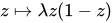
Benoît Mandelbrot, working at IBM's Thomas J. Watson Research Center, produced the first recognizable images of the set in late 1979 using the company's mainframe computers, marking a pivotal moment in visualizing complex iterative processes.[3] These high-resolution graphics, generated through extensive computational power available at IBM during the late 1970s and early 1980s, revealed the set's intricate fractal boundary and self-similar structures, transforming abstract mathematics into striking visual forms.[4] In December 1980, Mandelbrot published his seminal paper "Fractal Aspects of the Iteration of z → λz(1-z) for Complex λ and z" in the Annals of the New York Academy of Sciences, where he detailed the set's fractal properties and its connections to quadratic iterations.[15] This work built on his ongoing research at IBM since the 1970s, where he pioneered the use of computer graphics to explore fractal geometry, coining the term "fractal" in 1975 to describe such irregular, scale-invariant shapes.[4] The set, initially unnamed in Mandelbrot's publications, was formally dubbed the "Mandelbrot set" in the early 1980s by mathematicians Adrien Douady and John H. Hubbard in recognition of his visualizations.[3] Mandelbrot further popularized the set through his 1982 book The Fractal Geometry of Nature, which integrated the images and concepts into a broader framework for understanding natural irregularity, influencing fields beyond pure mathematics.[16] His IBM-era efforts in the 1970s and 1980s established fractals as a cornerstone of modern geometry, demonstrating how simple equations could yield boundless complexity.[4] The Mandelbrot set played a key role in popularizing chaos theory, serving as an iconic example of deterministic yet unpredictable systems, as highlighted in James Gleick's 1987 bestseller Chaos: Making a New Science.[4] Mandelbrot's contributions earned him the 2003 Japan Prize in Science and Technology for creating universal concepts in complex systems, including chaos and fractals.[16]Core Mathematical Properties
Fundamental Characteristics
The filled Mandelbrot set is compact, being a closed and bounded subset of the complex plane contained within the disk of radius 2 centered at the origin, as any orbit starting from |c| > 2 will escape to infinity under the iteration with .[14] It is also connected, a theorem established by Douady and Hubbard through the construction of a conformal isomorphism between the complement of the set and the exterior of the unit disk, ensuring no disconnection in the parameter space.[14] Moreover, the filled Mandelbrot set possesses a non-empty interior, comprising open regions called hyperbolic components where the quadratic map exhibits expanding dynamics away from attracting cycles.[14] Numerical computations indicate that the area of the filled Mandelbrot set is finite, approximately 1.50659 (as of 2025), though an exact closed-form expression remains unknown; recent estimates yield 1.50659189 ± 5×10^{-9}.[17] The boundary of the Mandelbrot set is a fractal curve with Hausdorff dimension exactly 2, a result proven by Shishikura via detailed study of the bifurcation loci and parabolic points on the boundary.[18] Central to the set's definition is the critical point 0, the unique finite critical point of the quadratic family ; membership in the filled Mandelbrot set requires the orbit of 0 to remain bounded, and within hyperbolic components—filling the interior—this orbit attracts to a stable periodic cycle, ensuring hyperbolicity of the dynamics for those parameters.[14]Hyperbolic Components and Bulbs
The hyperbolic components of the Mandelbrot set are the connected open subsets of its interior where the quadratic map possesses an attracting periodic cycle.[14] These components are simply connected regions homeomorphic to the unit disk, each corresponding to a fixed period of the attracting cycle, and they organize the set's internal structure through a tree-like hierarchy of attachments.[14] The main cardioid represents the period-1 hyperbolic component, centered at where the fixed point has multiplier 0, and bounded by a root at where the multiplier equals 1.[14] This component contains all parameters for which has a unique attracting fixed point, forming the largest bulb at the heart of the Mandelbrot set.[14] Attached to the boundary of the main cardioid are period- bulbs for , which are smaller hyperbolic components of period bifurcating from the cardioid at points where the fixed point's multiplier has period .[14] These bulbs are combinatorially labeled by rational internal angles in lowest terms, which determine their positions and the landing points of external rays on their roots; for instance, the prominent period-2 bulb attaches at the cusp of the cardioid with internal angle .[14] Misiurewicz points mark the boundaries of these bulbs, serving as parameters where the critical orbit (starting from 0) is strictly preperiodic, landing on a repelling cycle after finitely many iterations, and characterized by external arguments that are rational with even denominators.[14] Under the Douady-Hubbard theory, each hyperbolic component of period in the Mandelbrot set corresponds bijectively to an attracting cycle of period in the associated Julia set for , with the cycle's points varying holomorphically inside and the multiplier map (the unit disk) being a conformal isomorphism.[14] This establishes a fundamental link between the parameter space of the Mandelbrot set and the dynamics of individual quadratic maps.[14] The centers of these bulbs, particularly for perturbations within the period-1 framework, are given by the formulaBoundary Connectivity
The boundary of the Mandelbrot set exhibits intricate topological properties, central to which is the Mandelbrot Local Connectivity (MLC) conjecture proposed by Adrien Douady and John H. Hubbard in the 1980s. This conjecture asserts that the Mandelbrot set is locally connected, meaning that for every point on its boundary, there exists a basis of connected neighborhoods, which would imply that the boundary can be parametrized continuously by external angles via landing external rays.[14] Local connectivity remains unproven in full generality but has profound implications for understanding the set's structure, including the denseness of certain parameter rays and the separation of hyperbolic components.[19] Significant partial progress toward the MLC conjecture was achieved by Jean-Christophe Yoccoz in the late 1980s, who established local connectivity of the Mandelbrot set at parameters corresponding to quadratic irrationals, particularly those arising from quadratic polynomials with irrational indifferent fixed points of bounded type. Yoccoz's results relied on combinatorial tools like the Yoccoz puzzle, demonstrating local connectivity for finitely renormalizable parameters and linking it to the local connectivity of associated Julia sets.[20] Recent partial results include the proof by Dudko and Lyubich (2023) of local connectivity at satellite parameters of bounded type.[21] A key tool in analyzing boundary connectivity is the system of external rays, which are curves in the complement of the Mandelbrot set emanating from infinity and parameterized by angles in the unit circle. These rays land at boundary points, with rational angles guaranteed to land at rational preperiodic or periodic points, such as Misiurewicz points or roots of hyperbolic components, thereby providing a combinatorial parametrization of accessible boundary arcs. The landing behavior of these rays separates the parameter plane and supports partial connectivity results, as coincident landings at a point indicate local topological structure. Douady and Hubbard showed that at least two rays land at the critical point , and extensions confirm that every rational ray lands, facilitating the study of boundary access points.[14][22]Self-Similarity and Scaling
The Mandelbrot set exhibits profound self-similarity, characterized by the presence of infinitely many smaller copies, known as mini-Mandelbrots or baby Mandelbrot sets, embedded near its boundary. These mini-Mandelbrots appear as scaled and slightly distorted replicas of the full set, often attached to the main structure at points corresponding to hyperbolic components or Misiurewicz points. For instance, a prominent mini-Mandelbrot appears near the period-2 bulb at approximately $ c \approx -0.75 $, with scaling factors determined by renormalization theory; in period-doubling cascades, scalings are governed by the Feigenbaum constant , yielding ratios around . Similarly, other mini-Mandelbrots emerge with scaling factors such as , reflecting the iterative nature of the quadratic map $ z \mapsto z^2 + c $.[14] This self-similarity arises from the renormalization theory applied to quadratic dynamics, where successive period-doubling bifurcations produce nested structures governed by universal scaling exponents. In particular, the Feigenbaum constants describe these scalings: the parameter-scaling constant $ \delta \approx 4.67 $, which quantifies the ratio of distances between successive bifurcation points in the parameter space, and the spatial-scaling constant $ \alpha \approx 2.50 $, which governs the contraction of orbit sizes under renormalization. These constants, originally derived for real maps, extend to the complex plane in the Mandelbrot set, explaining the geometric shrinkage of mini-Mandelbrots during period-doubling cascades along real parameter slices. Douady and Hubbard adapted this framework to complex dynamics, showing how renormalization operators yield fixed points that mirror the set's fractal repetition.[4][23] The existence of infinitely many such small copies is rigorously proven through the landing of external rays on the set's boundary. For quadratic maps, Douady and Hubbard demonstrated that every external ray with rational argument lands at a boundary point, creating access points where mini-Mandelbrots bifurcate from the main set via conformal mappings and potential theory. This construction, using abstract Hubbard trees, ensures an infinite hierarchy of self-similar components without gaps, confirming the set's local connectivity in these regions.[14] Examples of self-similar features include the antennae—thin, branching filaments extending from bulbs—and the intricate filaments connecting hyperbolic components. These structures repeat at finer scales, with antennae displaying recursive spikes and curves that mimic larger boundary patterns, scaled down by factors tied to the eigenvalue of the indifferent fixed point in the associated Julia set. Such repetitions highlight the set's fractal dimension and its ties to renormalization fixed points.[14]Links to Julia Sets
The Mandelbrot set $ M $ functions as the connectedness locus for the Julia sets $ J_c $ arising from the quadratic polynomials $ f_c(z) = z^2 + c $, where $ c \in \mathbb{C} $. For any parameter $ c $, the Julia set $ J_c $ (the boundary of the filled Julia set $ K_c $) is connected if and only if $ c \in M $; otherwise, $ J_c $ is a totally disconnected Cantor set. This parameter-dynamics duality, establishing $ M $ as the bifurcation locus where connectivity transitions occur, was rigorously developed by Adrien Douady and John H. Hubbard in their foundational analysis of quadratic dynamics.[14][24] The critical role in this linkage is played by the orbit of the critical point 0 under iteration of $ f_c $, known as the critical orbit: $ z_0 = 0 $, $ z_1 = f_c(0) = c $, $ z_2 = f_c(c) = c^2 + c $, and so on. Membership of $ c $ in $ M $ is equivalent to this critical orbit remaining bounded, which guarantees that $ K_c $ is connected and thus $ J_c $ is connected. Conversely, if the critical orbit tends to infinity, $ K_c $ decomposes into a collection of disjoint quasidisks, leading to a disconnected $ J_c $. This criterion underscores how the boundedness of a single orbit in the dynamical plane determines the topological properties of $ J_c $ and parametrizes the structure of $ M $.[14][24] An illustrative example is the case $ c = 0 $, where $ f_0(z) = z^2 $ and the critical orbit is fixed at 0, remaining bounded. Here, the filled Julia set $ K_0 $ is the closed unit disk $ { z : |z| \leq 1 } $, and the Julia set $ J_0 $ is its boundary, the unit circle, both of which are connected. This configuration corresponds to a superattracting fixed point at 0 and exemplifies the central hyperbolic component of $ M $.[14] The Douady-Hubbard theorem solidifies these connections by proving that $ M $ itself is a compact, connected set in the complex plane, ensuring the coherence of the parameter space across all connected Julia sets.[24]Geometric Features
Main Cardioid and Periods
The main cardioid forms the central, heart-shaped region of the Mandelbrot set, corresponding to parameter values $ c $ for which the quadratic map $ f_c(z) = z^2 + c $ possesses an attracting fixed point.[14] This component is bounded by a smooth curve except at its cusp located at $ c = 0.25 $ on the real axis, where the fixed point becomes parabolic with multiplier 1, creating a sharp point due to the coalescence of two fixed points.[14] The cardioid's boundary is parametrized by the equation $ c(\theta) = \frac{\mu}{2} (1 - \frac{\mu}{2}) $, where $ \mu = e^{2\pi i \theta} $ and $ \theta \in [0, 1) $, derived from the condition that the fixed point $ z $ satisfies $ |2z| < 1 $ and $ c = z - z^2 $.[25] Visually, the cardioid exhibits rotational symmetry and serves as the primary outline, with numerous smaller bulbs symmetrically attached along its boundary, each representing regions of periodic attractors. Hyperbolic bulbs attach directly to the main cardioid at parabolic points on its boundary, where the multiplier of the cycle is a root of unity $ e^{2\pi i p/q} $ with $ p $ and $ q $ coprime.[14] These bulbs are hyperbolic components of period $ q $, and their attachment points mark bifurcations from the period-1 dynamics of the cardioid.[14] A prominent example is the period-2 bulb, attached at the parabolic point $ c = -0.75 $, forming a circular region centered near $ c = -1 $ where orbits converge to a 2-cycle.[25] Along the negative real axis, a period-doubling cascade emerges, with successively smaller bulbs of periods 4, 8, 16, and higher powers of 2 attaching to the period-2 bulb, illustrating the bifurcation sequence leading to chaotic dynamics beyond the set.[14] The intricate connections between the main cardioid and its bulbs are delineated by antennae—thin, fractal filaments extending from the cardioid's boundary—and external landing rays, which are curves in the parameter plane approaching the set from infinity.[14] These rays, parametrized by angles $ \theta \in \mathbb{Q}/\mathbb{Z} $, land precisely at parabolic points on the cardioid or bulb roots for periodic angles, with exactly two rays meeting at each such point to separate adjacent hyperbolic components.[26] For instance, rays at angles 0 and 1/2 land at the cusp $ c = 0.25 $, while rational angles with odd denominators target roots and even denominators target preperiodic Misiurewicz points along the antennae.[26] This ray structure provides a combinatorial framework for labeling and navigating the set's topology, emphasizing the cardioid's role as the hub of periodic organization.[14]Internal Structure and Zooming
Deep magnifications into the Mandelbrot set reveal an intricate internal structure characterized by thin filaments, spiraling patterns, and isolated Siegel disks. Filaments, often described as vein-like allowable arcs connecting hyperbolic components, form the delicate bridges between bulbs and exhibit extreme variability in shape and orientation, contributing to the set's topological complexity.[14] Spirals emerge prominently in bifurcation regions, where star-like structures with multiple branches appear, driven by the cyclic ordering of external rays landing on roots of components.[14] Siegel disks, which are linearizing domains around Diophantine indifferent periodic points, manifest as circular regions of quasi-conformal invariance within the set, surrounded by finer tendrils that persist under iteration.[14] Misiurewicz points, defined as parameters where the critical orbit becomes preperiodic—meaning the critical point 0 maps eventually to a repelling periodic cycle—mark specific locations of abrupt dynamical transitions in the set.[14] These points are strictly preperiodic and serve as landing sites for rational external rays with even-denominator arguments, influencing the local connectivity of the boundary.[14] A representative example is the Misiurewicz point at $ c \approx -0.1225 + 0.7449i $, where the critical orbit has preperiod 2 and period 3, leading to a finite post-critical set and hyperbolic dynamics outside the filled Julia set.[27] The boundary of the Mandelbrot set displays infinite complexity, with its Hausdorff dimension equal to 2, implying that while the set itself has finite area (approximately 1.50659), the boundary's one-dimensional Hausdorff measure—corresponding to length—is infinite.[28][1] This fractal dimension underscores the boundary's space-filling nature in local neighborhoods, where fine-scale features like filaments and spirals proliferate without bound. Recent numerical estimates as of September 2025 refine the area to approximately 1.506484 ± 0.000004.[29] Zoom sequences into the Mandelbrot set, achieved through high-precision computations, uncover recursive patterns of miniature copies and hyperbolic components at magnifications exceeding $ 10^{20} $. For instance, explorations near the main cardioid's boundary reveal nested spirals and filament networks that mirror larger-scale features, with each level of zoom exposing new layers of preperiodic points and indifferent cycles.[4] Such deep zooms require advanced rendering techniques to handle the exponential increase in iteration depth, highlighting the set's boundless detail.[4]Mathematical Constants in the Set
The Mandelbrot set exhibits intriguing connections to fundamental mathematical constants through its geometric and dynamical structure, particularly in the parameterization of external rays and the scaling properties of its components. External rays, which approach the boundary of the set from infinity, are parameterized by an angle $ \theta \in [0,1) $, corresponding to an argument of $ 2\pi \theta $ in the complex plane. Thus, the constant $ \pi $ inherently appears in these angular descriptions. For instance, the root point of the period-3 hyperbolic bulb, located in the wake between external rays at angles $ \theta = 1/3 $ and $ \theta = 2/3 $, is the landing point of rays at $ \theta = 1/7 $ and $ \theta = 2/7 $, yielding arguments $ 2\pi/7 $ and $ 4\pi/7 $.[30] These rays delineate the bulb's position relative to the main cardioid, highlighting $ \pi $'s role in the combinatorial organization of the set's hyperbolic components. The Fibonacci sequence also manifests in the Mandelbrot set through the periods of bulbs attached to the main cardioid. Starting from the primary bulbs of periods 1, 2, and 3, the sequence of periods for successively larger bulbs between them follows the Fibonacci numbers: 1, 2, 3, 5, 8, 13, and so on. This arises from the Farey tree structure governing bulb adjacencies, where the period of a bulb between periods $ p $ and $ q $ is $ p + q $. Consequently, the ratios of sizes (or "hyperbolic radii") of these successive bulbs approach the golden ratio $ \phi = (1 + \sqrt{5})/2 \approx 1.618 $, reflecting a scaling symmetry tied to the set's internal hierarchy.[30] In the period-doubling cascade along the real axis of the Mandelbrot set, the Feigenbaum constant $ \delta \approx 4.669201609102990671853203821578 $ governs the universal scaling behavior. This constant describes the limit of the ratios of distances between consecutive bifurcation points as periods double infinitely, converging to the Feigenbaum point at $ c \approx -1.401155189092 $. The same $ \delta $ appears in the geometric contraction of the "feathers" or substructures near this limit point, underscoring the universality of period-doubling transitions across quadratic maps.[31] Specific ray landings further embed constants like $ \pi $ in the set's topology. For example, the external ray at $ \theta = 1/5 $ (argument $ 2\pi/5 $) lands at a Misiurewicz point on the boundary, illustrating how rational angles with even denominators connect to preperiodic dynamics. While many such landings occur off the real axis, symmetric pairs of rays, such as those at $ \theta = 1/3 $ and $ 2/3 $ (arguments $ 2\pi/3 $), land at the parabolic root $ c = -3/4 $ on the real axis, marking the attachment of the period-2 bulb.[14]Extensions and Generalizations
Multibrot and Tricorn Sets
The Multibrot sets generalize the Mandelbrot set to polynomials of higher degree, defined as the connectedness locus of the family of maps $ f_c(z) = z^d + c $, where $ d > 2 $ is an integer and $ c \in \mathbb{C} $. Specifically, the Multibrot set of degree $ d $ consists of all complex parameters $ c $ for which the orbit of the critical point $ z_0 = 0 $ under iteration of $ f_c $ remains bounded.[32][33] These sets retain core topological properties of the Mandelbrot set, such as compactness and full connectivity, but display altered symmetries and greater structural intricacy as $ d $ increases. Unlike the quadratic case's bilateral reflection symmetry over the real axis, Multibrot sets exhibit $ (d-1) $-fold rotational symmetry around the origin, leading to $ (d-1) $ primary cardioids fused at their cusps in the main body. Higher degrees introduce more pronounced dendritic filaments and cusp formations in the boundary, enhancing the fractal complexity; for instance, the degree-4 Multibrot set features three joined cardioids with elaborate, tree-like appendages extending outward.[32][34][35] The tricorn set, sometimes called the Mandelbar set, provides another extension by incorporating complex conjugation in the quadratic iteration: $ f_c(z) = \overline{z}^2 + c $. It is the set of parameters $ c $ for which the corresponding filled Julia set remains connected, revealing a triangular outline with three prominent cusps and intricate interior bulbs. Distinct from the Multibrot family, the tricorn possesses order-3 rotational symmetry, arising from the anti-holomorphic dynamics, which results in a more radially symmetric yet topologically richer boundary than the standard Mandelbrot set.[36] Generalized multicorn sets extend this conjugation approach to higher degrees via $ f_c(z) = \overline{z}^d + c $, where the symmetry evolves to higher orders (often $ d+1 $-fold), yielding progressively complex connectedness loci with multiple symmetric lobes and heightened fractal detail. These structures, including the tricorn as the degree-2 case, are analyzed for their hyperbolic components and local connectivity, paralleling but diverging from holomorphic Multibrot dynamics in ways that highlight the role of reflection in fractal formation.[37]Higher-Dimensional Analogues
The quaternion Mandelbrot set generalizes the classical Mandelbrot set to four dimensions by performing the iteration $ z_{n+1} = z_n^2 + c $ where both $ z $ and $ c $ are quaternions, elements of the non-commutative division algebra over the reals.[38] The set consists of those $ c \in \mathbb{H} $ for which the sequence starting from $ z_0 = 0 $ remains bounded.[38] This extension was formalized using a matrix representation of quaternions to preserve the quadratic mapping's structure, revealing a connected set analogous to its complex counterpart but embedded in .[38] Non-commutativity in quaternion multiplication introduces significant challenges, as the order of factors affects the result, leading to path-dependent iterations and a proliferation of distinct slices when projecting the 4D set for visualization.[38] To render these sets, researchers typically fix one quaternion component (e.g., the scalar or one imaginary part) to obtain 3D or 2D views, such as volume renderings of the boundary where orbits escape to infinity. These slices often exhibit intricate, self-similar structures with increased topological complexity compared to the 2D case, including filaments and bulbs that vary across different projections. Further generalization to octonions yields an 8-dimensional analogue, iterating the same quadratic map over the [39] algebra, which is non-commutative and non-associative.[40] The loss of associativity complicates the dynamics, causing iterations to depend not only on the order of multiplication but also on parenthesization, resulting in even more fragmented and asymmetric sets.[40] Visualization in this case requires multi-dimensional slicing, often reducing to 3D hyperslices, which highlight the set's complex structure. An octonionic generalization of the Mandelbrot set has been proposed, sensitive to transition points due to non-associativity.[40] In the 2020s, advances in computational rendering have enabled high-resolution 3D visualizations of quaternion Mandelbrot slices using techniques like ray casting and voxel-based volume rendering, uncovering higher-genus surfaces in the boundaries that suggest richer topological features in higher dimensions. These renders, often incorporating memory-modified iterations for enhanced detail, demonstrate the set's volume scaling with parameters and provide insights into escape-time behaviors across 4D space.Non-Quadratic Mappings
The connectedness locus for the family of monic cubic polynomials $ f_{a,b}(z) = z^3 + a z + b $, often referred to as the cubic Mandelbrot set, consists of all parameters $ (a,b) \in \mathbb{C}^2 $ such that the corresponding Julia set $ J(f_{a,b}) $ is connected.[41] This locus is compact and connected, featuring a main hyperbolic component analogous to the main cardioid of the quadratic Mandelbrot set, but with additional substructure arising from the two distinct finite critical points, the roots of the derivative equation $ 3z^2 + a = 0 $ (i.e., $ z = \pm \sqrt{-a/3} $ when $ a < 0 $).[41] These critical points allow for more varied dynamical behaviors, such as independent periodic orbits, resulting in multiple secondary hyperbolic components and a higher genus surface when considering periodic parameter slices.[41] For transcendental mappings like the exponential family $ f_c(z) = e^z + c $, the parameter space is defined as the set of $ c \in \mathbb{C} $ for which the orbit of the singular critical value $ c $ remains bounded under iteration, forming a connected but unbounded region with infinitely many hyperbolic components and a fractal boundary featuring "hairs" or dynamic rays landing on the boundary.[42] Unlike polynomials, exponential maps have no finite critical points but feature an essential singularity at infinity and the asymptotic value $ c $ acting as a critical point.[42] The structure includes hyperbolic components corresponding to attracting periodic orbits of the singular value, exhibiting self-similar patterns reminiscent of quadratic dynamics but unbounded in extent.[42] Newton's method fractals arise as parameter spaces for rational maps derived from root-finding iterations of polynomials, such as cubics. For a cubic polynomial with three distinct roots, the Newton map $ N_p(z) = z - \frac{p(z)}{p'(z)} $ is a degree-3 rational function with three superattracting fixed points at the roots and one free critical point whose orbit determines connectivity.[43] The connectedness locus $ M_N $ in the parameter space (varying root positions) is the set of parameters where the filled Julia set (basins of attraction) is connected, and it admits homeomorphisms to the quadratic Mandelbrot set via quasi-conformal surgery on the basins.[43] This analogy highlights universal features in holomorphic dynamics, despite the higher degree and multiple attracting basins. A key property distinguishing non-quadratic mappings from the standard quadratic case is the presence of multiple critical points or singular values, which introduce additional degrees of freedom in orbit behavior and yield more components in the connectedness locus.[41][43] For instance, in cubics, the independent dynamics of the two critical points can create "captured" components where one critical orbit is periodic while the other escapes, expanding the topological complexity beyond the single-critical-point quadratic structure.[41] Similarly, the free critical point in Newton maps interacts with superattracting basins to produce decorations and bifurcations mirroring Mandelbrot-like hierarchies.[43] Examples of such mappings include perturbed quadratics of the form $ f_c(z) = z^2 + c z $, where the linear term shifts the critical point from zero, altering the parameter space while preserving quadratic degree; the connectedness locus remains homeomorphic to the standard Mandelbrot set via affine conjugation, but exhibits translated and scaled features.[24] These non-standard families illustrate how modifications to the quadratic form, even minor ones, can reveal analogous fractal boundaries without changing fundamental connectivity properties.Computation and Rendering
Rendering Algorithms
Rendering the Mandelbrot set at high magnifications requires sophisticated algorithms to manage the exponential increase in computational demands posed by deep zooms, where iteration counts can exceed billions and arbitrary-precision arithmetic is necessary to avoid numerical instability. Perturbation theory addresses this by selecting a reference point near the zoom center and computing its full orbit using high-precision arithmetic, then approximating the orbits of nearby pixels as small perturbations relative to this reference. This method leverages the fact that perturbations remain small over many iterations, allowing the use of lower-precision arithmetic for most pixels and reducing the overall computation time significantly for deep zooms.[44][45] Combining perturbation with series approximation further optimizes performance by representing the perturbed orbits as Taylor series expansions around the reference orbit, enabling the prediction and skipping of iterations until the approximation breaks down due to accumulated error. The series coefficients are precomputed once for the reference, and perturbations are applied per pixel, transforming the naive per-pixel iteration cost from quadratic in the number of iterations (across pixels, roughly ) to effectively linear or better in practice for suitable reference points. This hybrid approach has enabled zooms to magnifications exceeding , far beyond what standard escape-time methods can achieve efficiently.[44][46] Boundary tracing techniques complement these methods for initial renders or less extreme zooms by exploiting the topological properties of the set, where regions of uniform escape behavior are simply connected without enclaves. The algorithm starts from a known boundary point and traces contours by checking neighboring pixels' escape times, filling interior regions without full iteration counts and prioritizing boundary pixels that require more computation. In the 2020s, GPU-accelerated variants of boundary tracing combined with perturbation have been implemented to handle high-resolution deep zooms, achieving real-time previews at resolutions up to 16K using massive VRAM, such as 48 GB on NVIDIA RTX GPUs.[47][48][49] For applications demanding mathematical certainty, such as formal verification or high-stakes scientific visualization, interval arithmetic provides guaranteed renders by propagating bounds on complex values during iteration rather than point estimates. Each iteration operates on intervals for real and imaginary parts, ensuring that if the interval remains bounded within the disk of radius 2, the pixel is rigorously inside the set; otherwise, escape is confirmed without false positives from rounding errors. This method, while slower than floating-point approximations, enables exact classification at arbitrary precision.[50][51]Programming Implementations
The Mandelbrot set can be rendered using the escape-time algorithm in Python, leveraging libraries like NumPy for efficient array operations and Matplotlib for visualization. This approach iterates the quadratic map $ z_{n+1} = z_n^2 + c $ for each point $ c $ in a complex grid until $ |z_n| $ exceeds a threshold or a maximum iteration count is reached, coloring pixels based on the escape iteration. A representative implementation uses a grid of 1500 by 1250 points over the bounds from -2.25 to 0.75 in the real part and -1.25 to 1.25 in the imaginary part, with a maximum of 200 iterations for detail.[52] To enhance rendering quality, the iteration count is normalized and a power law (gamma=0.3) is applied to the colormap for smoother gradients, while shading via light sources adds depth. Vectorized NumPy computations handle the loops efficiently, replacing NaN values with zeros for stability, and the process takes approximately 3.7 seconds on standard hardware.[52] Below is the core code snippet adapted from this method:import numpy as np
import matplotlib.pyplot as plt
from matplotlib.colors import PowerNorm
from matplotlib.colors import LightSource
def mandelbrot(h, w, max_iter=200):
y, x = np.ogrid[-1.25:1.25:h*1j, -2.25:0.75:w*1j]
c = x + y*1j
z = c
divtime = max_iter + np.zeros(z.shape, dtype=int)
for i in range(max_iter):
z = z**2 + c
diverge = abs(z) > 4
div_now = diverge & (divtime == max_iter)
divtime[div_now] = i
z[diverge] = 4
return divtime
plt.imshow(mandelbrot(1250, 1500), cmap='hot', norm=PowerNorm(0.3), extent=[-2.25, 0.75, -1.25, 1.25])
ls = LightSource(315, 30)
plt.contourf(mandelbrot(1250, 1500), levels=20, cmap='hot', norm=PowerNorm(0.3), extend='both', alpha=0.5)
rgb = ls.shade(mandelbrot(1250, 1500), cmap='hot', norm=PowerNorm(0.3))
plt.imshow(rgb)
plt.show()
vec2 c = vec2(2.0) * (texcoords - 0.5) + vec2(0.0, 0.0);  // constant c, varies onscreen
vec2 z = c;
for (int i = 0; i < 15; i++) {
    if (z.r * z.r + z.g * z.g >= 4.0) break;
    z = vec2(z.r * z.r - z.g * z.g, 2.0 * z.r * z.g) + c;
}
gl_FragColor = fract(vec4(z.r, z.g, 0.25 * [length](/page/Length)(z), 0));