
Community hub
Recent from talks
Contribute something
Nothing was collected or created yet.
Nuclear shell model
View on Wikipedia
| Nuclear physics |
|---|
In nuclear physics, atomic physics, and nuclear chemistry, the nuclear shell model utilizes the Pauli exclusion principle to model the structure of atomic nuclei in terms of energy levels.[1] The first shell model was proposed by Dmitri Ivanenko (together with E. Gapon) in 1932. The model was developed in 1949 following independent work by several physicists, most notably Maria Goeppert Mayer and J. Hans D. Jensen, who received the 1963 Nobel Prize in Physics for their contributions to this model, and Eugene Wigner, who received the Nobel Prize alongside them for his earlier foundational work on atomic nuclei.[2]
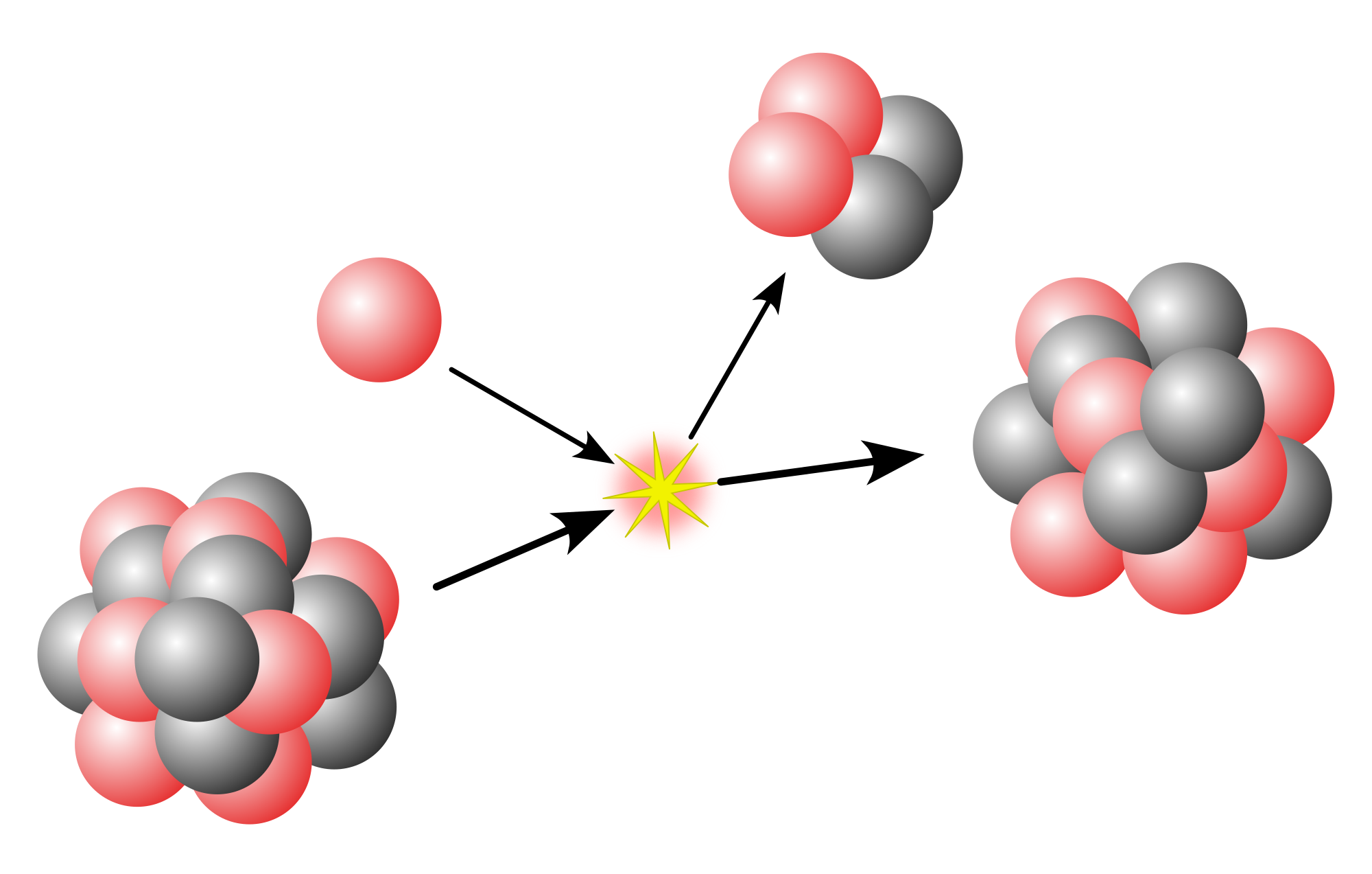
The nuclear shell model is partly analogous to the atomic shell model, which describes the arrangement of electrons in an atom, in that a filled shell results in better stability. When adding nucleons (protons and neutrons) to a nucleus, there are certain points where the binding energy of the next nucleon is significantly less than the last one. This observation that there are specific magic quantum numbers of nucleons (2, 8, 20, 28, 50, 82, and 126) that are more tightly bound than the following higher number is the origin of the shell model.
The shells for protons and neutrons are independent of each other. Therefore, there can exist both "magic nuclei", in which one nucleon type or the other is at a magic number, and "doubly magic quantum nuclei", where both are. Due to variations in orbital filling, the upper magic numbers are 126 and, speculatively, 184 for neutrons, but only 114 for protons, playing a role in the search for the so-called island of stability. Some semi-magic numbers have been found, notably Z = 40, which gives the nuclear shell filling for the various elements; 16 may also be a magic number.[3]
To get these numbers, the nuclear shell model starts with an average potential with a shape somewhere between the square well and the harmonic oscillator. To this potential, a spin-orbit term is added. Even so, the total perturbation does not coincide with the experiment, and an empirical spin-orbit coupling must be added with at least two or three different values of its coupling constant, depending on the nuclei being studied.


The magic numbers of nuclei, as well as other properties, can be arrived at by approximating the model with a three-dimensional harmonic oscillator plus a spin–orbit interaction. A more realistic but complicated potential is known as the Woods–Saxon potential.
Modified harmonic oscillator model
[edit]Consider a three-dimensional harmonic oscillator. This would give, for example, in the first three levels ("ℓ" is the angular momentum quantum number):
| level n | ℓ | mℓ | ms |
|---|---|---|---|
| 0 | 0 | 0 | +1/2 |
| −1/2 | |||
| 1 | 1 | +1 | +1/2 |
| −1/2 | |||
| 0 | +1/2 | ||
| −1/2 | |||
| −1 | +1/2 | ||
| −1/2 | |||
| 2 | 0 | 0 | +1/2 |
| −1/2 | |||
| 2 | +2 | +1/2 | |
| −1/2 | |||
| +1 | +1/2 | ||
| −1/2 | |||
| 0 | +1/2 | ||
| −1/2 | |||
| −1 | +1/2 | ||
| −1/2 | |||
| −2 | +1/2 | ||
| −1/2 |
Nuclei are built by adding protons and neutrons. These will always fill the lowest available level, with the first two protons filling level zero, the next six protons filling level one, and so on. As with electrons in the periodic table, protons in the outermost shell will be relatively loosely bound to the nucleus if there are only a few protons in that shell because they are farthest from the center of the nucleus. Therefore, nuclei with a full outer proton shell will have a higher nuclear binding energy than other nuclei with a similar total number of protons. The same is true for neutrons.
This means that the magic numbers are expected to be those in which all occupied shells are full. In accordance with the experiment, we get 2 (level 0 full) and 8 (levels 0 and 1 full) for the first two numbers. However, the full set of magic numbers does not turn out correctly. These can be computed as follows:
- In a three-dimensional harmonic oscillator the total degeneracy of states at level n is .
- Due to the spin, the degeneracy is doubled and is .
- Thus, the magic numbers would befor all integer k. This gives the following magic numbers: 2, 8, 20, 40, 70, 112, ..., which agree with experiment only in the first three entries. These numbers are twice the tetrahedral numbers (1, 4, 10, 20, 35, 56, ...) from the Pascal Triangle.


In particular, the first six shells are:
- level 0: 2 states (ℓ = 0) = 2.
- level 1: 6 states (ℓ = 1) = 6.
- level 2: 2 states (ℓ = 0) + 10 states (ℓ = 2) = 12.
- level 3: 6 states (ℓ = 1) + 14 states (ℓ = 3) = 20.
- level 4: 2 states (ℓ = 0) + 10 states (ℓ = 2) + 18 states (ℓ = 4) = 30.
- level 5: 6 states (ℓ = 1) + 14 states (ℓ = 3) + 22 states (ℓ = 5) = 42.
where for every ℓ there are 2ℓ+1 different values of ml and 2 values of ms, giving a total of 4ℓ+2 states for every specific level.
These numbers are twice the values of triangular numbers from the Pascal Triangle: 1, 3, 6, 10, 15, 21, ....
Including a spin-orbit interaction
[edit]We next include a spin–orbit interaction. First, we have to describe the system by the quantum numbers j, mj and parity instead of ℓ, ml and ms, as in the hydrogen–like atom. Since every even level includes only even values of ℓ, it includes only states of even (positive) parity. Similarly, every odd level includes only states of odd (negative) parity. Thus we can ignore parity in counting states. The first six shells, described by the new quantum numbers, are
- level 0 (n = 0): 2 states (j = 1/2). Even parity.
- level 1 (n = 1): 2 states (j = 1/2) + 4 states (j = 3/2) = 6. Odd parity.
- level 2 (n = 2): 2 states (j = 1/2) + 4 states (j = 3/2) + 6 states (j = 5/2) = 12. Even parity.
- level 3 (n = 3): 2 states (j = 1/2) + 4 states (j = 3/2) + 6 states (j = 5/2) + 8 states (j = 7/2) = 20. Odd parity.
- level 4 (n = 4): 2 states (j = 1/2) + 4 states (j = 3/2) + 6 states (j = 5/2) + 8 states (j = 7/2) + 10 states (j = 9/2) = 30. Even parity.
- level 5 (n = 5): 2 states (j = 1/2) + 4 states (j = 3/2) + 6 states (j = 5/2) + 8 states (j = 7/2) + 10 states (j = 9/2) + 12 states (j = 11/2) = 42. Odd parity.
where for every j there are 2j+1 different states from different values of mj.
Due to the spin–orbit interaction, the energies of states of the same level but with different j will no longer be identical. This is because in the original quantum numbers, when is parallel to , the interaction energy is positive, and in this case j = ℓ + s = ℓ + 1/2. When is anti-parallel to (i.e. aligned oppositely), the interaction energy is negative, and in this case j=ℓ−s=ℓ−1/2. Furthermore, the strength of the interaction is roughly proportional to ℓ.


For example, consider the states at level 4:
- The 10 states with j = 9/2 come from ℓ = 4 and s parallel to ℓ. Thus they have a positive spin–orbit interaction energy.
- The 8 states with j = 7/2 came from ℓ = 4 and s anti-parallel to ℓ. Thus they have a negative spin–orbit interaction energy.
- The 6 states with j = 5/2 came from ℓ = 2 and s parallel to ℓ. Thus they have a positive spin–orbit interaction energy. However, its magnitude is half compared to the states with j = 9/2.
- The 4 states with j = 3/2 came from ℓ = 2 and s anti-parallel to ℓ. Thus they have a negative spin–orbit interaction energy. However, its magnitude is half compared to the states with j = 7/2.
- The 2 states with j = 1/2 came from ℓ = 0 and thus have zero spin–orbit interaction energy.
Changing the profile of the potential
[edit]The harmonic oscillator potential grows infinitely as the distance from the center r goes to infinity. A more realistic potential, such as the Woods–Saxon potential, would approach a constant at this limit. One main consequence is that the average radius of nucleons' orbits would be larger in a realistic potential. This leads to a reduced term in the Laplace operator of the Hamiltonian operator. Another main difference is that orbits with high average radii, such as those with high n or high ℓ, will have a lower energy than in a harmonic oscillator potential. Both effects lead to a reduction in the energy levels of high ℓ orbits.


Predicted magic numbers
[edit]
Together with the spin–orbit interaction, and for appropriate magnitudes of both effects, one is led to the following qualitative picture: at all levels, the highest j states have their energies shifted downwards, especially for high n (where the highest j is high). This is both due to the negative spin–orbit interaction energy and to the reduction in energy resulting from deforming the potential into a more realistic one. The second-to-highest j states, on the contrary, have their energy shifted up by the first effect and down by the second effect, leading to a small overall shift. The shifts in the energy of the highest j states can thus bring the energy of states of one level closer to the energy of states of a lower level. The "shells" of the shell model are then no longer identical to the levels denoted by n, and the magic numbers are changed.
We may then suppose that the highest j states for n = 3 have an intermediate energy between the average energies of n = 2 and n = 3, and suppose that the highest j states for larger n (at least up to n = 7) have an energy closer to the average energy of n−1. Then we get the following shells (see the figure)
- 1st shell: 2 states (n = 0, j = 1/2).
- 2nd shell: 6 states (n = 1, j = 1/2 or 3/2).
- 3rd shell: 12 states (n = 2, j = 1/2, 3/2 or 5/2).
- 4th shell: 8 states (n = 3, j = 7/2).
- 5th shell: 22 states (n = 3, j = 1/2, 3/2 or 5/2; n = 4, j = 9/2).
- 6th shell: 32 states (n = 4, j = 1/2, 3/2, 5/2 or 7/2; n = 5, j = 11/2).
- 7th shell: 44 states (n = 5, j = 1/2, 3/2, 5/2, 7/2 or 9/2; n = 6, j = 13/2).
- 8th shell: 58 states (n = 6, j = 1/2, 3/2, 5/2, 7/2, 9/2 or 11/2; n = 7, j = 15/2).
and so on.
Note that the numbers of states after the 4th shell are doubled triangular numbers plus two. Spin–orbit coupling causes so-called "intruder levels" to drop down from the next higher shell into the structure of the previous shell. The sizes of the intruders are such that the resulting shell sizes are themselves increased to the next higher doubled triangular numbers from those of the harmonic oscillator. For example, 1f2p has 20 nucleons, and spin–orbit coupling adds 1g9/2 (10 nucleons), leading to a new shell with 30 nucleons. 1g2d3s has 30 nucleons, and adding intruder 1h11/2 (12 nucleons) yields a new shell size of 42, and so on.
The magic numbers are then
- 2
- 8=2+6
- 20=2+6+12
- 28=2+6+12+8
- 50=2+6+12+8+22
- 82=2+6+12+8+22+32
- 126=2+6+12+8+22+32+44
- 184=2+6+12+8+22+32+44+58
and so on. This gives all the observed magic numbers and also predicts a new one (the so-called island of stability) at the value of 184 (for protons, the magic number 126 has not been observed yet, and more complicated theoretical considerations predict the magic number to be 114 instead).
Another way to predict magic (and semi-magic) numbers is by laying out the idealized filling order (with spin–orbit splitting but energy levels not overlapping). For consistency, s is split into j = 1/2 and j = −1/2 components with 2 and 0 members respectively. Taking the leftmost and rightmost total counts within sequences bounded by / here gives the magic and semi-magic numbers.
- s(2,0)/p(4,2) > 2,2/6,8, so (semi)magic numbers 2,2/6,8
- d(6,4):s(2,0)/f(8,6):p(4,2) > 14,18:20,20/28,34:38,40, so 14,20/28,40
- g(10,8):d(6,4):s(2,0)/h(12,10):f(8,6):p(4,2) > 50,58,64,68,70,70/82,92,100,106,110,112, so 50,70/82,112
- i(14,12):g(10,8):d(6,4):s(2,0)/j(16,14):h(12,10):f(8,6):p(4,2) > 126,138,148,156,162,166,168,168/184,198,210,220,228,234,238,240, so 126,168/184,240
The rightmost predicted magic numbers of each pair within the quartets bisected by / are double tetrahedral numbers from the Pascal Triangle: 2, 8, 20, 40, 70, 112, 168, 240 are 2x 1, 4, 10, 20, 35, 56, 84, 120, ..., and the leftmost members of the pairs differ from the rightmost by double triangular numbers: 2 − 2 = 0, 8 − 6 = 2, 20 − 14 = 6, 40 − 28 = 12, 70 − 50 = 20, 112 − 82 = 30, 168 − 126 = 42, 240 − 184 = 56, where 0, 2, 6, 12, 20, 30, 42, 56, ... are 2 × 0, 1, 3, 6, 10, 15, 21, 28, ... .
Other properties of nuclei
[edit]This model also predicts or explains with some success other properties of nuclei, in particular spin and parity of nuclei ground states, and to some extent their excited nuclear states as well. Take 17
8O (oxygen-17) as an example: Its nucleus has eight protons filling the first three proton "shells", eight neutrons filling the first three neutron "shells", and one extra neutron. All protons in a complete proton shell have zero total angular momentum, since their angular momenta cancel each other. The same is true for neutrons. All protons in the same level (n) have the same parity (either +1 or −1), and since the parity of a pair of particles is the product of their parities, an even number of protons from the same level (n) will have +1 parity. Thus, the total angular momentum of the eight protons and the first eight neutrons is zero, and their total parity is +1. This means that the spin (i.e. angular momentum) of the nucleus, as well as its parity, are fully determined by that of the ninth neutron. This one is in the first (i.e. lowest energy) state of the 4th shell, which is a d-shell (ℓ = 2), and since p = (−1)ℓ, this gives the nucleus an overall parity of +1. This 4th d-shell has a j = 5/2, thus the nucleus of 17
8O is expected to have positive parity and total angular momentum 5/2, which indeed it has.
The rules for the ordering of the nucleus shells are similar to Hund's Rules of the atomic shells, however, unlike its use in atomic physics, the completion of a shell is not signified by reaching the next n, as such the shell model cannot accurately predict the order of excited nuclei states, though it is very successful in predicting the ground states. The order of the first few terms are listed as follows: 1s, 1p3/2, 1p1/2, 1d5/2, 2s, 1d3/2... For further clarification on the notation refer to the article on the Russell–Saunders term symbol.
For nuclei farther from the magic quantum numbers one must add the assumption that due to the relation between the strong nuclear force and total angular momentum, protons or neutrons with the same n tend to form pairs of opposite angular momentum. Therefore, a nucleus with an even number of protons and an even number of neutrons has 0 spin and positive parity. A nucleus with an even number of protons and an odd number of neutrons (or vice versa) has the parity of the last neutron (or proton), and the spin equal to the total angular momentum of this neutron (or proton). By "last" we mean the properties coming from the highest energy level.
In the case of a nucleus with an odd number of protons and an odd number of neutrons, one must consider the total angular momentum and parity of both the last neutron and the last proton. The nucleus parity will be a product of theirs, while the nucleus spin will be one of the possible results of the sum of their angular momenta (with other possible results being excited states of the nucleus).
The ordering of angular momentum levels within each shell is according to the principles described above – due to spin–orbit interaction, with high angular momentum states having their energies shifted downwards due to the deformation of the potential (i.e. moving from a harmonic oscillator potential to a more realistic one). For nucleon pairs, however, it is often energetically favourable to be at high angular momentum, even if its energy level for a single nucleon would be higher. This is due to the relation between angular momentum and the strong nuclear force.
The nuclear magnetic moment of neutrons and protons is partly predicted by this simple version of the shell model. The magnetic moment is calculated through j, ℓ and s of the "last" nucleon, but nuclei are not in states of well-defined ℓ and s. Furthermore, for odd-odd nuclei, one has to consider the two "last" nucleons, as in deuterium. Therefore, one gets several possible answers for the nuclear magnetic moment, one for each possible combined ℓ and s state, and the real state of the nucleus is a superposition of them. Thus the real (measured) nuclear magnetic moment is somewhere in between the possible answers.
The electric dipole of a nucleus is always zero, because its ground state has a definite parity. The matter density (ψ2, where ψ is the wavefunction) is always invariant under parity. This is usually the situation with the atomic electric dipole.
Higher electric and magnetic multipole moments cannot be predicted by this simple version of the shell model for reasons similar to those in the case of deuterium.
Including residual interactions
[edit]
For nuclei having two or more valence nucleons (i.e. nucleons outside a closed shell), a residual two-body interaction must be added. This residual term comes from the part of the inter-nucleon interaction not included in the approximative average potential. Through this inclusion, different shell configurations are mixed, and the energy degeneracy of states corresponding to the same configuration is broken.[5][6]
These residual interactions are incorporated through shell model calculations in a truncated model space (or valence space). This space is spanned by a basis of many-particle states where only single-particle states in the model space are active. The Schrödinger equation is solved on this basis, using an effective Hamiltonian specifically suited for the model space. This Hamiltonian is different from the one of free nucleons as, among other things, it has to compensate for excluded configurations.[6]
One can do away with the average potential approximation entirely by extending the model space to the previously inert core and treating all single-particle states up to the model space truncation as active. This forms the basis of the no-core shell model, which is an ab initio method. It is necessary to include a three-body interaction in such calculations to achieve agreement with experiments.[7]
Collective rotation and the deformed potential
[edit]In 1953 the first experimental examples were found of rotational bands in nuclei, with their energy levels following the same J(J+1) pattern of energies as in rotating molecules. Quantum mechanically, it is impossible to have a collective rotation of a sphere, so this implied that the shape of these nuclei was non-spherical. In principle, these rotational states could have been described as coherent superpositions of particle-hole excitations in the basis consisting of single-particle states of the spherical potential. But in reality, the description of these states in this manner is intractable, due to a large number of valence particles—and this intractability was even greater in the 1950s when computing power was extremely rudimentary. For these reasons, Aage Bohr, Ben Mottelson, and Sven Gösta Nilsson constructed models in which the potential was deformed into an ellipsoidal shape. The first successful model of this type is now known as the Nilsson model. It is essentially the harmonic oscillator model described in this article, but with anisotropy added, so the oscillator frequencies along the three Cartesian axes are not all the same. Typically the shape is a prolate ellipsoid, with the axis of symmetry taken to be z. Because the potential is not spherically symmetric, the single-particle states are not states of good angular momentum J. However, a Lagrange multiplier , known as a "cranking" term, can be added to the Hamiltonian. Usually the angular frequency vector ω is taken to be perpendicular to the symmetry axis, although tilted-axis cranking can also be considered. Filling the single-particle states up to the Fermi level produces states whose expected angular momentum along the cranking axis is the desired value.


Related models
[edit]Igal Talmi developed a method to obtain the information from experimental data and use it to calculate and predict energies which have not been measured. This method has been successfully used by many nuclear physicists and has led to a deeper understanding of nuclear structure. The theory which gives a good description of these properties was developed. This description turned out to furnish the shell model basis of the elegant and successful interacting boson model.
A model derived from the nuclear shell model is the alpha particle model developed by Henry Margenau, Edward Teller, J. K. Pering, T. H. Skyrme, also sometimes called the Skyrme model.[8][9] Note, however, that the Skyrme model is usually taken to be a model of the nucleon itself, as a "cloud" of mesons (pions), rather than as a model of the nucleus as a "cloud" of alpha particles.
See also
[edit]References
[edit]- ^ "Shell Model of Nucleus". HyperPhysics.
- ^ Nobel Lectures, Physics 1963-1970. Amsterdam, Netherlands: Elsevier Publishing Company. 1972. Retrieved May 19, 2023.
- ^ Ozawa, A.; Kobayashi, T.; Suzuki, T.; Yoshida, K.; Tanihata, I. (2000). "New Magic Number, N=16, near the Neutron Drip Line". Physical Review Letters. 84 (24): 5493–5. Bibcode:2000PhRvL..84.5493O. doi:10.1103/PhysRevLett.84.5493. PMID 10990977. (this refers to the nuclear drip line)
- ^ Wang, Meng; Audi, G.; Kondev, F. G.; Huang, W.J.; Naimi, S.; Xu, Xing (March 2017). "The AME2016 atomic mass evaluation (II). Tables, graphs and references". Chinese Physics C. 41 (3) 030003. Bibcode:2017ChPhC..41c0003W. doi:10.1088/1674-1137/41/3/030003. hdl:11858/00-001M-0000-0010-23E8-5. ISSN 1674-1137.
- ^ Caurier, E.; Martínez-Pinedo, G.; Nowacki, F.; Poves, A.; Zuker, A. P. (2005). "The shell model as a unified view of nuclear structure". Reviews of Modern Physics. 77 (2): 427–488. arXiv:nucl-th/0402046. Bibcode:2005RvMP...77..427C. doi:10.1103/RevModPhys.77.427. S2CID 119447053.
- ^ a b Coraggio, L.; Covello, A.; Gargano, A.; Itaco, N.; Kuo, T.T.S. (2009). "Shell-model calculations and realistic effective interactions". Progress in Particle and Nuclear Physics. 62 (1): 135–182. arXiv:0809.2144. Bibcode:2009PrPNP..62..135C. doi:10.1016/j.ppnp.2008.06.001. S2CID 18722872.
- ^ Barrett, B. R.; Navrátil, P.; Vary, J. P. (2013). "Ab initio no core shell model". Progress in Particle and Nuclear Physics. 69: 131–181. arXiv:0902.3510. Bibcode:2013PrPNP..69..131B. doi:10.1016/j.ppnp.2012.10.003.
- ^ Skyrme, T. H. R. (February 7, 1961). "A Non-Linear Field Theory". Proceedings of the Royal Society A: Mathematical, Physical and Engineering Sciences. 260 (1300): 127–138. Bibcode:1961RSPSA.260..127S. doi:10.1098/rspa.1961.0018. S2CID 122604321.
- ^ Skyrme, T. H. R. (March 1962). "A unified field theory of mesons and baryons". Nuclear Physics. 31: 556–569. Bibcode:1962NucPh..31..556S. doi:10.1016/0029-5582(62)90775-7.
Further reading
[edit]- Talmi, Igal; de-Shalit, A. (1963). Nuclear Shell Theory. Academic Press. ISBN 978-0-486-43933-4.
{{cite book}}: ISBN / Date incompatibility (help) - Talmi, Igal (1993). Simple Models of Complex Nuclei: The Shell Model and the Interacting Boson Model. Harwood Academic Publishers. ISBN 978-3-7186-0551-4.
External links
[edit]- Igal Talmi (November 24, 2010). On single nucleon wave functions. RIKEN Nishina Center.
Nuclear shell model
View on GrokipediaHistorical Development
Early Ideas (1930s)
The discovery of the neutron by James Chadwick in 1932 marked a pivotal moment in nuclear physics, enabling the conceptualization of the atomic nucleus as a composite of protons and neutrons rather than protons and electrons. This development, occurring amid the rapid advancement of quantum mechanics, prompted early explorations into the internal structure of nuclei, drawing analogies to the layered electron configurations in atoms. In August 1932, shortly after the neutron's identification, Soviet physicists Dmitri Ivanenko and E. Gapon proposed the first rudimentary shell model for the nucleus. They suggested that protons and neutrons occupy discrete energy levels, filling them sequentially in a manner akin to electrons in atomic orbitals, governed by the Pauli exclusion principle. This independent particle approximation aimed to explain nuclear stability and binding energies but lacked detailed potential specifications, serving primarily as a qualitative framework.[5] Building on these ideas, Werner Heisenberg advanced the concept in his 1932 paper, emphasizing short-range exchange forces between nucleons to achieve saturation in nuclear binding. Heisenberg argued that such forces would lead to filled energy shells, promoting stability when certain numbers of protons or neutrons completed orbital fillings, thus providing a mechanism for shell-like organization without long-range Coulomb effects dominating. His isotopic spin formalism treated protons and neutrons symmetrically, reinforcing the viability of layered nucleon arrangements.[6] Early efforts to quantify these levels, often using simple potentials like the harmonic oscillator without spin-orbit coupling, resulted in predicted shell closures at nucleon numbers such as 20 and 40. For instance, calculations based on a three-dimensional oscillator potential yielded degeneracies leading to these values as stable configurations, but they failed to match observed stabilities at 20 and 50, highlighting the limitations of the pre-1940s models. These attempts, pursued by researchers including Ivanenko and others, demonstrated periodicities in binding energies but required later refinements for accuracy.[7]Mayer-Jensen Formulation (1949)
In 1949, Maria Goeppert Mayer and J. Hans D. Jensen independently developed the nuclear shell model by incorporating a strong spin-orbit interaction into the independent particle framework, successfully explaining the observed nuclear magic numbers of 2, 8, 20, and 28. Mayer's formulation appeared in Physical Review as a letter emphasizing the role of spin-orbit coupling in splitting degenerate orbital levels, while Jensen, collaborating with Otto Haxel and Hans Suess, published a concurrent letter in the same journal detailing similar insights derived from analyzing nuclear binding energies and angular momenta. The key insight of their work was that a large spin-orbit term inverts the energy ordering within subshells, particularly for p-states where the level (with total angular momentum ) lies below the level (), enabling shell closures at the observed magic numbers. This inversion arises because the spin-orbit interaction favors aligned spin and orbital angular momentum, lowering the energy of states with higher . Without this coupling, the harmonic oscillator potential alone predicts shell closures at 2, 8, 20, and 40, failing to match experiment; with it, the splitting groups levels to yield closures at 2 (filling ), 8 (adding and ), 20 (including , , and ), and 28 (incorporating the lowered subshell). The spin-orbit Hamiltonian term introduced by Mayer and Jensen is given by where ensures an attractive interaction, is the orbital angular momentum operator, and is the spin operator. Using the identity , this term shifts the energy of states downward by and states upward by , with the splitting magnitude increasing for higher . Their initial predictions demonstrated that this modification to the three-dimensional harmonic oscillator levels resolves discrepancies with experimental data on stable isotopes and binding energies, establishing the shell model as a cornerstone of nuclear structure theory.Nobel Recognition and Refinements
The nuclear shell model gained widespread recognition through the 1963 Nobel Prize in Physics, awarded jointly to Maria Goeppert Mayer and J. Hans D. Jensen for their independent development of the model, which explained the structure of atomic nuclei in terms of quantized energy shells for protons and neutrons.[2] This accolade highlighted the model's success in accounting for magic numbers and nuclear stability, marking a pivotal validation of independent-particle approaches in nuclear physics. In the 1950s, experimental evidence strongly corroborated the shell model's predictions, particularly in beta decay processes and nuclear magnetic moments. Measurements of beta decay spectra and log ft values for odd-A nuclei aligned closely with shell model expectations for allowed transitions, as outlined by Nordheim's selection rules, which linked decay rates to single-particle configurations and confirmed shell closures at magic numbers like 28 and 50.[8] Similarly, observed magnetic moments of odd-mass nuclei near closed shells matched the Schmidt limits derived from the model, with deviations in other cases attributable to configuration mixing, further solidifying the framework's predictive power. Early refinements to the model addressed limitations in reproducing fine details of energy level splittings and multipole moments. Adjustments to the strength of the spin-orbit coupling term improved fits to spectroscopic data across isotopic chains, while the inclusion of tensor forces in the effective nucleon-nucleon interaction accounted for perturbations in shell fillings and enhanced agreement with binding energies in light nuclei.[9] These modifications, explored in calculations during the mid-1950s, preserved the core independent-particle approximation while incorporating realistic two-body effects. Eugene Wigner's contributions to symmetry principles in nuclear structure provided a theoretical bridge between the microscopic shell model and macroscopic collective descriptions, facilitating the unified model of Bohr and Mottelson.[10] By applying group theory to classify nuclear states and interactions, Wigner's supermultiplet scheme connected single-particle orbitals to emergent rotational and vibrational behaviors in deformed nuclei, enabling a more comprehensive understanding of nuclear dynamics beyond closed shells.[2]Fundamental Concepts
Analogy to Atomic Electron Shells
The nuclear shell model draws a direct conceptual parallel to the atomic shell model developed in quantum mechanics for electrons, where individual particles occupy discrete energy levels determined by solving the Schrödinger equation in a central potential. In the nuclear context, protons and neutrons—collectively known as nucleons—likewise fill quantized energy states within an average nuclear potential, leading to shell-like structures that explain patterns of nuclear stability. This analogy was historically motivated by the success of the atomic model in accounting for the periodic table of elements, prompting physicists in the mid-20th century to adapt similar principles to the nucleus despite the challenges posed by the strong nuclear force.[11][12] Key similarities between the two models include the filling of shells with particles up to a maximum capacity, resulting in closed-shell configurations that exhibit exceptional stability. Just as noble gases in atomic physics have filled electron shells and thus low reactivity, nuclei with "magic" numbers of protons or neutrons—such as 2, 8, 20, 28, 50, 82, or 126—display enhanced binding energies and resistance to decay or capture processes. The quantum numbers governing these levels are analogous as well: the principal quantum number , orbital angular momentum , total angular momentum , and magnetic projections play comparable roles in labeling states and enforcing occupancy limits via the Pauli exclusion principle.[13] Despite these parallels, significant differences arise due to the distinct physics of the nuclear interior. The atomic model relies on the long-range electromagnetic force from the positively charged nucleus acting on electrons, whereas the nuclear shell model operates under the short-range strong nuclear force binding nucleons, which lacks the scaling (where is the atomic number) seen in atomic energies. Additionally, protons and neutrons are treated as distinct particles occupying separate but similar shell systems, often formalized through isospin symmetry where they represent two states of the nucleon (isospin up for protons, down for neutrons), unlike the identical electrons in atoms. These adaptations were crucial in the model's formulation to reconcile nuclear data with atomic-inspired ideas.[11][12]Independent Particle Approximation
The independent particle approximation forms the cornerstone of the nuclear shell model, positing that the total wave function of the nucleus can be represented as a Slater determinant constructed from single-particle orbitals occupied up to the Fermi level, thereby neglecting two-body correlations in the initial formulation.[14] This antisymmetric product of one-body wave functions ensures compliance with the Pauli exclusion principle while simplifying the many-body Schrödinger equation into a set of independent single-particle equations.[15] In this approach, the ground state is obtained by filling the lowest-energy orbitals with protons and neutrons separately, reflecting the isospin distinction between these fermions.[14] Central to this approximation is the mean-field concept, wherein each nucleon experiences an average potential generated by the distribution of all other nucleons in the nucleus, analogous to the Hartree-Fock method in atomic physics where electrons move in the field averaged over the charge density of their peers.[15] This effective potential captures the collective influence of the nuclear many-body system, allowing nucleons to be treated as quasi-independent particles whose motions are governed by a self-consistent field.[14] The seminal formulation by Mayer and Jensen in 1949 introduced this framework to explain nuclear magic numbers and stability, building on earlier ideas of closed shells. The validity of the independent particle approximation is justified by the short-range nature of the strong nuclear force, which limits interactions to nearby nucleons and promotes saturation of nuclear binding energy at a constant density of approximately 0.16 fm⁻³, akin to a liquid drop where local correlations dominate but do not disrupt the overall mean-field picture.[15] This short-range character results in a large mean free path for nucleons—often comparable to or exceeding nuclear dimensions—indicating infrequent collisions and supporting the assumption of nearly independent motion.[14] Furthermore, the approximation is empirically supported by the density of single-particle states near the Fermi level, where observed spectroscopic properties, such as excitation energies and magnetic moments, align closely with predictions from mean-field solutions, as validated in Brueckner theory for nuclear matter.[15] While effective for describing ground-state properties and low-lying excitations, the independent particle approximation has inherent limitations, as real nuclei exhibit correlations beyond the mean field that require residual interactions for a complete description.[14]Role of the Pauli Exclusion Principle
In the nuclear shell model, protons and neutrons are treated as fermions with half-integer spin, each type obeying the Pauli exclusion principle independently due to their distinct electric charges, which prevents them from occupying the same quantum state. This fermionic nature ensures that no two identical nucleons can share the same set of quantum numbers, leading to a quantized distribution of particles across discrete energy levels analogous to electron configurations in atoms. The principle is foundational to the independent particle approximation, where nucleons move in a mean-field potential generated by all others.[16][17] Within each subshell characterized by total angular momentum (where is the orbital angular momentum), the Pauli principle limits occupancy to a maximum of nucleons, corresponding to the possible projections of along a quantization axis. This degeneracy arises from the distinct magnetic quantum numbers , allowing one nucleon per state while respecting antisymmetry of the wave function. Protons and neutrons fill their respective subshells separately, though the isospin formalism recognizes their near-identical behavior under the strong nuclear force, treating them as two states of the nucleon isospin doublet with symmetric single-particle potentials in the absence of Coulomb effects.[16][17][18] The filling sequence proceeds by populating the lowest-energy subshells first, adhering strictly to Pauli-allowed occupancies, which results in closed shells when all states in a major shell are fully occupied. This sequential buildup minimizes the total energy and enforces shell structure, with protons and neutrons each contributing to their own closures. For even-even nuclei, where both proton and neutron numbers are even, the ground state features total angular momentum , as paired nucleons in time-reversed states couple to zero spin and parity, forming a stable configuration without unpaired particles.[17][16][18] Excitation spectra in the shell model arise primarily from particle-hole promotions, where a nucleon is excited from a filled subshell (creating a hole) to an empty higher subshell, in full compliance with the Pauli principle to avoid double occupancy. These transitions generate low-lying states with specific selection rules, such as changes in parity and angular momentum dictated by the single-particle operators, and underscore the principle's role in dictating nuclear stability and response to perturbations.[17][16]Basic Single-Particle Model
Three-Dimensional Harmonic Oscillator
In the nuclear shell model, the three-dimensional isotropic harmonic oscillator potential provides a foundational approximation for the mean-field experienced by individual nucleons, enabling the derivation of basic single-particle energy levels. The potential takes the form where is the nucleon mass and is the angular frequency of oscillation. This quadratic potential confines nucleons within a nuclear volume and yields analytically solvable energy levels that are equally spaced in multiples of , facilitating the identification of shell structures without the complexities of more realistic potentials.[19] The quantum mechanical treatment of this potential separates into three independent one-dimensional oscillators along the Cartesian axes, resulting in energy eigenvalues expressed as where is the total oscillator quantum number, is the principal radial quantum number, and is the orbital angular momentum quantum number (with limited to even or odd values depending on ). The associated magnetic quantum number takes integer values from to . States sharing the same exhibit degeneracy, forming discrete major shells; for instance, the ground shell consists solely of the state (, ), accommodating 2 nucleons when spin is included, while the shell comprises the states (, ), with orbital degeneracy of 3 and total capacity of 6 nucleons including spin degeneracy. The orbital degeneracy for a given is , reflecting the number of possible combinations summing to .[19] To align the model with experimental nuclear sizes, the oscillator frequency parameter is empirically tuned such that MeV, where is the mass number of the nucleus. This scaling ensures the spatial extent of the wave functions, characterized by the oscillator length , matches the nuclear radius fm, thereby reproducing the overall energy scale of single-particle excitations on the order of 10–20 MeV for typical nuclei.[20]Quantum Numbers and Energy Levels
In the basic single-particle nuclear shell model, employing the three-dimensional isotropic harmonic oscillator potential, individual nucleon states are specified by five quantum numbers: the principal quantum number (total number of oscillator quanta), the radial quantum number (number of radial nodes), the orbital angular momentum quantum number (with corresponding to s, p, d, f, etc.), the total angular momentum quantum number (accounting for the nucleon's spin of ), and the projection quantum number (ranging from to in integer steps). These labels parallel those in atomic physics but adapt to the nuclear mean field, where protons and neutrons occupy separate but analogous sets of levels due to the Pauli exclusion principle, allowing up to two nucleons (one of each isospin) per state. Without residual interactions or spin-orbit coupling, the energy levels are highly degenerate within each major shell defined by , as the energy depends solely on and is independent of , , , and . The subshell ordering within a shell follows increasing , but all states in a given shell share the same energy, leading to large degeneracies that accommodate multiple nucleons. The lowest-energy sequence begins with the shell (, , ), followed by (, , ; , , ), (, , ; , , ; , , ), and (, , ; , , ; , , ; , , ). The degeneracy of each subshell is given by , yielding total states per major shell of . The following table summarizes the first few major shells, their subshells, and degeneracies:| Major Shell | Subshells | Total States per Shell | Cumulative States |
|---|---|---|---|
| 0 | 2 | 2 | |
| 1 | , | 6 | 8 |
| 2 | , , | 12 | 20 |
| 3 | , , , | 20 | 40 |