Polarization density
Main page
2159599

Polarization density

logo
Community Hub0 subscribers
Read side by side
from Wikipedia

In classical electromagnetism, polarization density (or electric polarization, or simply polarization) is the vector field that expresses the volumetric density of permanent or induced electric dipole moments in a dielectric material. When a dielectric is placed in an external electric field, its molecules gain electric dipole moment and the dielectric is said to be polarized.

Electric polarization of a given dielectric material sample is defined as the quotient of electric dipole moment (a vector quantity, expressed as coulombs*meters (C*m) in SI units) to volume (meters cubed).[1][2] Polarization density is denoted mathematically by P;[2] in SI units, it is expressed in coulombs per square meter (C/m2).

Polarization density also describes how a material responds to an applied electric field as well as the way the material changes the electric field, and can be used to calculate the forces that result from those interactions. It can be compared to magnetization, which is the measure of the corresponding response of a material to a magnetic field in magnetism.

Similar to ferromagnets, which have a non-zero permanent magnetization even if no external magnetic field is applied, ferroelectric materials have a non-zero polarization in the absence of external electric field.

Definition

[edit]

An external electric field that is applied to a dielectric material, causes a displacement of bound charged elements.

A bound charge is a charge that is associated with an atom or molecule within a material. It is called "bound" because it is not free to move within the material like free charges. Positive charged elements are displaced in the direction of the field, and negative charged elements are displaced opposite to the direction of the field. The molecules may remain neutral in charge, yet an electric dipole moment forms.[3][4]

For a certain volume element in the material, which carries a dipole moment , we define the polarization density P:

In general, the dipole moment changes from point to point within the dielectric. Hence, the polarization density P of a dielectric inside an infinitesimal volume dV with an infinitesimal dipole moment dp is:

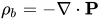
The net charge appearing as a result of polarization is called bound charge and denoted .

This definition of polarization density as a "dipole moment per unit volume" is widely adopted, though in some cases it can lead to ambiguities and paradoxes.[5]

Other expressions

[edit]

Let a volume dV be isolated inside the dielectric. Due to polarization the positive bound charge will be displaced a distance relative to the negative bound charge , giving rise to a dipole moment . Substitution of this expression in (1) yields

Since the charge bounded in the volume dV is equal to the equation for P becomes:[3]

where is the density of the bound charge in the volume under consideration. It is clear from the definition above that the dipoles are overall neutral and thus is balanced by an equal density of opposite charges within the volume. Charges that are not balanced are part of the free charge discussed below.

Gauss's law for the field of P

[edit]

For a given volume V enclosed by a surface S, the bound charge inside it is equal to the flux of P through S taken with the negative sign, or

Proof

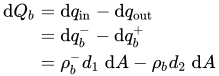
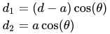
Let a surface area S envelope part of a dielectric. Upon polarization negative and positive bound charges will be displaced. Let d1 and d2 be the distances of the bound charges and , respectively, from the plane formed by the element of area dA after the polarization. And let dV1 and dV2 be the volumes enclosed below and above the area dA.

Above: an elementary volume dV = dV1+ dV2 (bounded by the element of area dA) so small, that the dipole enclosed by it can be thought as that produce by two elementary opposite charges. Below, a planar view (click in the image to enlarge).

It follows that the negative bound charge moved from the outer part of the surface dA inwards, while the positive bound charge moved from the inner part of the surface outwards.


By the law of conservation of charge the total bound charge left inside the volume after polarization is:

Since and (see image to the right)

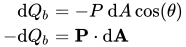
The above equation becomes

By (2) it follows that , so we get:

And by integrating this equation over the entire closed surface S we find that

\oiint

which completes the proof.

Differential form

[edit]

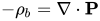
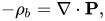
By the divergence theorem, Gauss's law for the field P can be stated in differential form as: where ∇ · P is the divergence of the field P through a given surface containing the bound charge density .
Proof

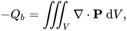
By the divergence theorem we have that for the volume V containing the bound charge . And since is the integral of the bound charge density taken over the entire volume V enclosed by S, the above equation yields which is true if and only if

Relationship between the fields of P and E

[edit]

Homogeneous, isotropic dielectrics

[edit]
Field lines of the D-field in a dielectric sphere with greater susceptibility than its surroundings, placed in a previously uniform field.[6] The field lines of the E-field are not shown: These point in the same directions, but many field lines start and end on the surface of the sphere, where there is bound charge. As a result, the density of E-field lines is lower inside the sphere than outside, which corresponds to the fact that the E-field is weaker inside the sphere than outside.

In a homogeneous, linear, non-dispersive and isotropic dielectric medium, the polarization is aligned with and proportional to the electric field E:[7]

where ε0 is the electric constant, and χ is the electric susceptibility of the medium. Note that in this case χ simplifies to a scalar, although more generally it is a tensor. This is a particular case due to the isotropy of the dielectric.

Taking into account this relation between P and E, equation (3) becomes:[3]

\oiint

The expression in the integral is Gauss's law for the field E which yields the total charge, both free and bound , in the volume V enclosed by S.[3] Therefore,

which can be written in terms of free charge and bound charge densities (by considering the relationship between the charges, their volume charge densities and the given volume):
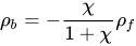
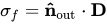
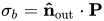
Since within a homogeneous dielectric there can be no free charges , by the last equation it follows that there is no bulk bound charge in the material . And since free charges can get as close to the dielectric as to its topmost surface, it follows that polarization only gives rise to surface bound charge density (denoted to avoid ambiguity with the volume bound charge density ).[3]

may be related to P by the following equation:[8] where is the normal vector to the surface S pointing outwards. (see charge density for the rigorous proof)
Anisotropic dielectrics

[edit]

The class of dielectrics where the polarization density and the electric field are not in the same direction are known as anisotropic materials.

In such materials, the i-th component of the polarization is related to the j-th component of the electric field according to:[7]
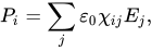
This relation shows, for example, that a material can polarize in the x direction by applying a field in the z direction, and so on. The case of an anisotropic dielectric medium is described by the field of crystal optics.

As in most electromagnetism, this relation deals with macroscopic averages of the fields and dipole density, so that one has a continuum approximation of the dielectric materials that neglects atomic-scale behaviors. The polarizability of individual particles in the medium can be related to the average susceptibility and polarization density by the Clausius–Mossotti relation.

In general, the susceptibility is a function of the frequency ω of the applied field. When the field is an arbitrary function of time t, the polarization is a convolution of the Fourier transform of χ(ω) with the E(t). This reflects the fact that the dipoles in the material cannot respond instantaneously to the applied field, and causality considerations lead to the Kramers–Kronig relations.

If the polarization P is not linearly proportional to the electric field E, the medium is termed nonlinear and is described by the field of nonlinear optics. To a good approximation (for sufficiently weak fields, assuming no permanent dipole moments are present), P is usually given by a Taylor series in E whose coefficients are the nonlinear susceptibilities:

where is the linear susceptibility, is the second-order susceptibility (describing phenomena such as the Pockels effect, optical rectification and second-harmonic generation), and is the third-order susceptibility (describing third-order effects such as the Kerr effect and electric field-induced optical rectification).

In ferroelectric materials, there is no one-to-one correspondence between P and E at all because of hysteresis.

Polarization density in Maxwell's equations

[edit]

The behavior of electric fields (E, D), magnetic fields (B, H), charge density (ρ) and current density (J) are described by Maxwell's equations in matter.

Relations between E, D and P

[edit]

In terms of volume charge densities, the free charge density is given by

where is the total charge density. By considering the relationship of each of the terms of the above equation to the divergence of their corresponding fields (of the electric displacement field D, E and P in that order), this can be written as:[9]


This is known as the constitutive equation for electric fields. Here ε0 is the electric permittivity of empty space. In this equation, P is the (negative of the) field induced in the material when the "fixed" charges, the dipoles, shift in response to the total underlying field E, whereas D is the field due to the remaining charges, known as "free" charges.[5][10]

In general, P varies as a function of E depending on the medium, as described later in the article. In many problems, it is more convenient to work with D and the free charges than with E and the total charge.[1]

Therefore, a polarized medium, by way of Green's theorem can be split into four components.

  • The bound volumetric charge density:
  • The bound surface charge density:
  • The free volumetric charge density:
  • The free surface charge density:

Time-varying polarization density

[edit]

When the polarization density changes with time, the time-dependent bound-charge density creates a polarization current density of

so that the total current density that enters Maxwell's equations is given by
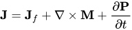
where Jf is the free-charge current density, and the second term is the magnetization current density (also called the bound current density), a contribution from atomic-scale magnetic dipoles (when they are present).

Polarization ambiguity

[edit]
Example of how the polarization density in a bulk crystal is ambiguous. (a) A solid crystal. (b) By pairing the positive and negative charges in a certain way, the crystal appears to have an upward polarization. (c) By pairing the charges differently, the crystal appears to have a downward polarization.

Crystalline materials

[edit]

In a simple approach the polarization inside a solid is not, in general, uniquely defined. Because a bulk solid is periodic, one must choose a unit cell in which to compute the polarization (see figure).[11][12] In other words, two people, Alice and Bob, looking at the same solid, may calculate different values of P, and neither of them will be wrong. For example, if Alice chooses a unit cell with positive ions at the top and Bob chooses the unit cell with negative ions at the top, their computed P vectors will have opposite directions. Alice and Bob will agree on the microscopic electric field E in the solid, but disagree on the value of the displacement field .

Even though the value of P is not uniquely defined in a bulk solid, variations in P are uniquely defined.[11] If the crystal is gradually changed from one structure to another, there will be a current inside each unit cell, due to the motion of nuclei and electrons. This current results in a macroscopic transfer of charge from one side of the crystal to the other, and therefore it can be measured with an ammeter (like any other current) when wires are attached to the opposite sides of the crystal. The time-integral of the current is proportional to the change in P. The current can be calculated in computer simulations (such as density functional theory); the formula for the integrated current turns out to be a type of Berry's phase.[11]

The non-uniqueness of P is not problematic, because every measurable consequence of P is in fact a consequence of a continuous change in P.[11] For example, when a material is put in an electric field E, which ramps up from zero to a finite value, the material's electronic and ionic positions slightly shift. This changes P, and the result is electric susceptibility (and hence permittivity). As another example, when some crystals are heated, their electronic and ionic positions slightly shift, changing P. The result is pyroelectricity. In all cases, the properties of interest are associated with a change in P.

In what is now called the modern theory of polarization, the polarization is defined as a difference. Any structure which has inversion symmetry has zero polarization; there is an identical distribution of positive and negative charges about an inversion center. If the material deforms there can be a polarization due to the charge in the charge distribution.[12]

Amorphous materials

[edit]

Another problem in the definition of P is related to the arbitrary choice of the "unit volume", or more precisely to the system's scale.[5] For example, at microscopic scale a plasma can be regarded as a gas of free charges, thus P should be zero. On the contrary, at a macroscopic scale the same plasma can be described as a continuous medium, exhibiting a permittivity and thus a net polarization P0.

See also

[edit]

References and notes

[edit]
[edit]
Revisions and contributorsEdit on WikipediaRead on Wikipedia
from Grokipedia
Polarization density, denoted as the vector field P\mathbf{P}, is a fundamental concept in classical electromagnetism representing the electric dipole moment per unit volume within a dielectric material exposed to an electric field.[1] It quantifies the extent to which the material's atoms or molecules become polarized, either through the alignment of permanent dipoles or the induction of temporary dipoles, resulting in a net separation of positive and negative charges.[2] Mathematically, P\mathbf{P} is expressed as P=Np\mathbf{P} = N \mathbf{p}, where NN is the number density of polarizable entities and p\mathbf{p} is the average dipole moment per entity, with units of coulombs per square meter in the SI system.[1] This polarization leads to the formation of bound charges, which are charges tied to the material's structure and do not move freely, distinguishing them from free charges.[2] The volume density of bound charge is given by ρb=P\rho_b = -\nabla \cdot \mathbf{P}, arising from spatial variations in P\mathbf{P}, while surface bound charge density appears at interfaces as σb=Pn^\sigma_b = \mathbf{P} \cdot \hat{\mathbf{n}}, where n^\hat{\mathbf{n}} is the outward normal vector.[1] These bound charges modify the total electric field inside the material, typically reducing it compared to the applied field in linear dielectrics.[2] In the framework of Maxwell's equations, polarization density is incorporated through the electric displacement field D=ϵ0E+P\mathbf{D} = \epsilon_0 \mathbf{E} + \mathbf{P}, where ϵ0\epsilon_0 is the vacuum permittivity and E\mathbf{E} is the electric field.[1] This leads to Gauss's law in the form D=ρf\nabla \cdot \mathbf{D} = \rho_f, where ρf\rho_f is the free charge density, simplifying calculations by isolating the effects of free charges from bound ones.[2] For linear isotropic dielectrics, P=ϵ0χeE\mathbf{P} = \epsilon_0 \chi_e \mathbf{E}, with χe\chi_e as the electric susceptibility, yielding D=ϵE\mathbf{D} = \epsilon \mathbf{E} where ϵ=ϵ0(1+χe)\epsilon = \epsilon_0 (1 + \chi_e) is the permittivity.[1] Polarization density plays a crucial role in applications such as capacitors, where it enhances capacitance by a factor of the relative permittivity, and in devices like electret microphones that exploit permanent polarization.[1] It also influences wave propagation in materials, affecting phenomena like birefringence and the behavior of electromagnetic waves in dielectrics.[2] Understanding P\mathbf{P} is essential for modeling the response of materials to electric fields in fields ranging from electronics to photonics.[1]

Fundamentals

Definition

Polarization density, denoted as the vector field P\vec{P}, quantifies the electric dipole moment per unit volume within a dielectric material exposed to an electric field. The electric dipole moment p\vec{p} of a localized distribution of charges is defined as p=iqiri\vec{p} = \sum_i q_i \vec{r}_i, where qiq_i are the charges and ri\vec{r}_i are their position vectors relative to a chosen origin within the distribution.[3] In dielectrics, an applied electric field causes a slight separation of positive and negative charges in atoms or molecules, inducing such dipole moments that align predominantly with the field.[4] Macroscopically, P(r)\vec{P}(\vec{r}) at a point r\vec{r} is obtained through spatial averaging of the microscopic dipole contributions over a small volume VV surrounding r\vec{r}, where VV is large enough to encompass many dipoles but small compared to variations in the field:
P(r)=1VVp(r)dV, \vec{P}(\vec{r}) = \frac{1}{V} \int_V \vec{p}(\vec{r}') \, dV',
with p(r)\vec{p}(\vec{r}') representing the local dipole moment density from all charges in the infinitesimal element dVdV'.[5] This averaging smooths out microscopic fluctuations to yield a continuous vector field describing the material's overall response. The SI units of P\vec{P} are coulombs per square meter (C/m²), reflecting its equivalence to a surface charge density.[6]

Microscopic Interpretation

Polarization density originates at the atomic and molecular scales through the formation of electric dipoles within materials exposed to an external electric field. In atoms, this begins with the displacement of electron clouds relative to the positively charged nuclei, creating induced atomic dipoles that contribute to the overall polarization.[7] This electron displacement is a universal mechanism in insulators, where the applied field distorts the symmetric charge distribution, leading to a net dipole moment per atom.[8] Several distinct mechanisms drive these microscopic dipoles, categorized by the nature of the material and the response to the field. Electronic polarization involves the aforementioned shift of electron clouds and occurs in all dielectrics, dominating at high frequencies. Atomic, or ionic, polarization arises in ionic crystals through the relative displacement of oppositely charged ions in the lattice, such as in sodium chloride (NaCl), where Na⁺ and Cl⁻ ions shift slightly under the field, enhancing the dipole density.[7] Orientational polarization occurs in materials with permanent molecular dipoles, like water (H₂O), where the asymmetric charge distribution allows the molecules to rotate and align with the field, overcoming thermal randomization.[8] Interfacial polarization, also known as space-charge polarization, emerges at boundaries or heterostructures due to the accumulation of mobile charges, creating effective dipoles at interfaces rather than within bulk atoms.[7] The total polarization density combines contributions from induced dipoles, which form solely due to the external field distorting charge distributions (as in electronic and atomic mechanisms), and permanent dipoles, which exist intrinsically but require field-induced alignment (as in orientational polarization). Induced dipoles are temporary and proportional to the field strength, while permanent ones rely on molecular structure for their baseline moment.[9] In water, for instance, the permanent dipole of each H₂O molecule (arising from oxygen's electronegativity) aligns to produce significant orientational effects at low frequencies, whereas NaCl's response is primarily from induced ionic shifts without inherent dipoles.[7] The microscopic view transitions to the macroscopic polarization density through statistical averaging over large ensembles of these dipoles, particularly in non-uniform fields where local variations must be smoothed to yield bulk properties. This averaging accounts for thermal fluctuations and spatial inhomogeneities, defining the observable polarization as an ensemble average rather than individual dipole moments.[10] Such an approach highlights limitations in directly equating microscopic behaviors to macroscopic observables without considering these statistical effects.[11]

Mathematical Formulations

Equivalent Expressions

One equivalent mathematical representation of the polarization density arises from microscopic charge distributions in dielectrics. For a localized, neutral charge configuration, the local polarization at position r\mathbf{r} can be expressed as an integral over the charge density ρ(r)\rho(\mathbf{r}') within a small volume surrounding r\mathbf{r}:
P(r)=(rr)ρ(r)dV, \mathbf{P}(\mathbf{r}) = \int \left( \mathbf{r}' - \mathbf{r} \right) \rho(\mathbf{r}') \, dV',
where the integral captures the effective dipole contribution from the displaced charges, assuming higher-order multipoles are negligible. This form is equivalent to the standard dipole-per-volume definition under the dipole approximation and is particularly useful for deriving macroscopic properties from atomic-scale charge arrangements./03%3A_Polarization_and_Conduction/3.01%3A_Polarization) An alternative integral expression emphasizes the dynamic origin of polarization through adiabatic charge transport. In this view, the polarization density is given by the space-time integral of the current density j(r,λ)\mathbf{j}(\mathbf{r}, \lambda) over an adiabatic parameter λ\lambda (typically from 0 to 1, representing a transition between reference states):
P(r)=01j(r,λ)dλ. \mathbf{P}(\mathbf{r}) = \int_0^1 \mathbf{j}(\mathbf{r}, \lambda) \, d\lambda.
This formulation, rooted in classical electrodynamics, treats polarization as the accumulated charge flow during a reversible deformation of the charge distribution and holds equivalence to static dipole models for slow, quasistatic processes. It clarifies ambiguities in finite systems and extends naturally to non-periodic structures.[12] In linear media, a differential form expresses the polarization density locally through the electric susceptibility χ\chi, where P(r)\mathbf{P}(\mathbf{r}) is proportional to the susceptibility at each point, reflecting spatial variations without explicit field dependence in the expression itself. This local, point-wise relation assumes isotropy and linearity, providing a continuum description suitable for inhomogeneous materials.[13] For periodic structures, such as crystals, Fourier transform representations facilitate computation via Bloch wavefunctions. The electronic contribution to polarization is obtained by integrating the Berry connection over the Brillouin zone:
Pel=e(2π)3ImnBZdkunkkunk, P_{el} = \frac{e}{(2\pi)^3} \mathrm{Im} \sum_n \int_{BZ} d\mathbf{k} \, \langle u_{n\mathbf{k}} | \nabla_{\mathbf{k}} u_{n\mathbf{k}} \rangle,
where unku_{n\mathbf{k}} are periodic parts of Bloch functions, summed over occupied bands nn, and the total polarization includes ionic terms. This k-space integral yields a multi-valued polarization modulo lattice vectors, essential for quantifying spontaneous polarization in ferroelectrics.[11] In computational simulations, polarization density is modeled either discretely or continuously. Discrete approaches assign inducible point dipoles to atomic sites, computing P\mathbf{P} as a sum over these moments divided by local volumes, which is efficient for molecular dynamics but approximates distributed charge effects. Continuous models, conversely, derive P\mathbf{P} from integrated electron or force densities across the simulation cell, offering higher fidelity for delocalized systems like solids, though at greater computational cost. These methods converge under refined grids, with discrete variants suiting large-scale polarizable force fields.[14]

Associated Bound Charges

In dielectrics, spatial variations in the polarization density P\mathbf{P} give rise to bound charges, which are immobile charges resulting from the displacement of electrons relative to positive nuclei within the material. These bound charges effectively act as sources of the electric field produced by the polarization itself, distinct from free charges that can move through the material.[15] The volume bound charge density ρb\rho_b is defined as
ρb=P, \rho_b = -\nabla \cdot \mathbf{P},
where the negative sign arises because a positive divergence of P\mathbf{P} corresponds to a net outflow of dipole moment, leaving an effective negative charge density.[16] To derive this, consider the scalar potential ϕP\phi_P generated by the dipole distribution equivalent to P\mathbf{P}:
ϕP(r)=14πϵ0VP(r)(rr)rr3dV. \phi_P(\mathbf{r}) = \frac{1}{4\pi\epsilon_0} \int_V \frac{\mathbf{P}(\mathbf{r}') \cdot (\mathbf{r} - \mathbf{r}')}{|\mathbf{r} - \mathbf{r}'|^3} \, dV'.
This integral can be transformed using the identity P(1/rr)=(P/rr)(P)/rr\mathbf{P} \cdot \nabla' (1/|\mathbf{r} - \mathbf{r}'|) = \nabla' \cdot (\mathbf{P}/|\mathbf{r} - \mathbf{r}'|) - (\nabla' \cdot \mathbf{P})/|\mathbf{r} - \mathbf{r}'| and integration by parts, yielding a volume term 14πϵ0VP(r)rrdV\frac{1}{4\pi\epsilon_0} \int_V \frac{-\nabla' \cdot \mathbf{P}(\mathbf{r}')}{|\mathbf{r} - \mathbf{r}'|} \, dV' plus surface contributions. The volume term matches the Coulomb potential from a charge density ρb=P\rho_b = -\nabla \cdot \mathbf{P}, so 2ϕP=ρb/ϵ0\nabla^2 \phi_P = -\rho_b / \epsilon_0. The associated electric field EP=ϕP\mathbf{E}_P = -\nabla \phi_P then satisfies Gauss's law in the form EP=ρb/ϵ0\nabla \cdot \mathbf{E}_P = \rho_b / \epsilon_0.[15] At the surface of the dielectric, a surface bound charge density σb\sigma_b forms due to the abrupt termination of P\mathbf{P}, given by
σb=Pn^, \sigma_b = \mathbf{P} \cdot \hat{\mathbf{n}},
where n^\hat{\mathbf{n}} is the outward-pointing unit normal vector. This term originates from the surface integral in the integration by parts of the potential derivation, representing the component of P\mathbf{P} normal to the boundary.[16] Physically, the divergence P\nabla \cdot \mathbf{P} quantifies a local imbalance in the density of aligned dipoles: a positive divergence implies more dipole flux leaving a volume than entering, equivalent to a net negative bound charge accumulation, while a negative divergence indicates a net positive bound charge accumulation. This dipole imbalance mimics the effect of separated positive and negative charges without actual charge transfer.[4] For uniform P\mathbf{P}, P=0\nabla \cdot \mathbf{P} = 0, so ρb=0\rho_b = 0 everywhere, but σb=P\sigma_b = P on one surface and σb=P\sigma_b = -P on the opposite surface, as seen in a uniformly polarized slab or cylinder. In contrast, non-uniform P\mathbf{P} in electrets—materials exhibiting quasi-permanent polarization due to frozen dipole alignments—produces both volume and surface bound charges, resulting in internal electric fields that persist over time.[16][15]

Field Relationships

Isotropic Dielectrics

In isotropic dielectrics, the polarization density P\mathbf{P} exhibits a linear and direction-independent response to the applied electric field E\mathbf{E}, characteristic of homogeneous materials where properties are uniform in all directions. This scalar relationship arises in media such as gases, liquids, and amorphous solids, where microscopic dipoles align without preferred orientations.[17] The constitutive relation for such materials is given by P=ϵ0χE\mathbf{P} = \epsilon_0 \chi \mathbf{E}, where ϵ0\epsilon_0 is the vacuum permittivity and χ\chi is the electric susceptibility, a scalar quantity that quantifies the material's ability to become polarized. This equation assumes a linear response, valid for sufficiently weak fields where higher-order effects are negligible.[17][18] This macroscopic relation derives from microscopic averaging in uniform media, where the polarization density P\mathbf{P} is the volume average of individual dipole moments pi\mathbf{p}_i from atoms or molecules: P=np\mathbf{P} = n \langle \mathbf{p} \rangle, with nn as the number density of polarizable units and p\langle \mathbf{p} \rangle the ensemble average dipole moment induced by the local field. In isotropic cases, each dipole responds linearly as p=αEloc\mathbf{p} = \alpha \mathbf{E}_\text{loc}, with α\alpha the atomic polarizability, leading to χ=nα/ϵ0\chi = n \alpha / \epsilon_0 after averaging over a volume much larger than molecular scales but smaller than macroscopic variations.[18] The permittivity ϵ\epsilon of the material connects directly to this relation via ϵ=ϵ0(1+χ)\epsilon = \epsilon_0 (1 + \chi), where the dielectric constant κ=1+χ\kappa = 1 + \chi measures the enhancement of capacitance relative to vacuum. For example, distilled water has κ80\kappa \approx 80 at room temperature, implying a high χ79\chi \approx 79, while dry air has κ1.0006\kappa \approx 1.0006 with χ0.0006\chi \approx 0.0006, reflecting weak polarization in dilute gases.[17] In practice, χ\chi exhibits frequency dependence due to resonant responses of bound charges, causing dispersion where the effective permittivity varies with the field's oscillation rate, though the linear form holds quasi-statically for non-resonant frequencies. This model is limited to linear, homogeneous conditions, failing in nonlinear regimes at strong fields or in inhomogeneous media where spatial variations disrupt uniform averaging.[17]

Anisotropic Dielectrics

In anisotropic dielectrics, the polarization density P\mathbf{P} does not align uniformly with the electric field E\mathbf{E} as in isotropic materials, where a scalar susceptibility χ\chi yields P=ϵ0χE\mathbf{P} = \epsilon_0 \chi \mathbf{E}; instead, the response depends on the direction of E\mathbf{E} relative to the material's crystal structure, leading to direction-dependent polarization.[19] This anisotropy arises from the lack of spherical symmetry in the atomic or molecular arrangement, requiring a tensor description to capture the varying polarizability along different axes.[20] The relationship between polarization and electric field is expressed using the electric susceptibility tensor χ\boldsymbol{\chi}, a 3×3 matrix, as
Pi=ϵ0χijEj, P_i = \epsilon_0 \chi_{ij} E_j,
where summation over repeated indices jj is implied, ϵ0\epsilon_0 is the vacuum permittivity, and the Einstein summation convention applies.[19] The tensor χ\boldsymbol{\chi} is symmetric (χij=χji\chi_{ij} = \chi_{ji}) due to the real nature of the dielectric response in non-absorbing media, and its components determine how P\mathbf{P} components arise from E\mathbf{E}.[20] The corresponding relative permittivity tensor is then ϵij/ϵ0=δij+χij\epsilon_{ij}/\epsilon_0 = \delta_{ij} + \chi_{ij}, where δij\delta_{ij} is the Kronecker delta, linking the displacement field D=ϵ0E+P\mathbf{D} = \epsilon_0 \mathbf{E} + \mathbf{P} to E\mathbf{E} via Di=ϵijEjD_i = \epsilon_{ij} E_j.[21] For practical analysis, the susceptibility tensor can be diagonalized by choosing coordinates aligned with the material's principal axes, simplifying χ\boldsymbol{\chi} to a diagonal form with elements χ1,χ2,χ3\chi_1, \chi_2, \chi_3 along these axes.[20] In uniaxial crystals, two principal susceptibilities are equal (χ1=χ2χ3\chi_1 = \chi_2 \neq \chi_3), corresponding to a single optic axis, while biaxial crystals have three distinct values (χ1χ2χ3\chi_1 \neq \chi_2 \neq \chi_3), with two optic axes.[21] A representative example is calcite (CaCOX3\ce{CaCO3}), a uniaxial crystal where the differing principal permittivities cause double refraction: an incident light ray splits into ordinary and extraordinary rays with orthogonal polarizations, experiencing refractive indices no1.658n_o \approx 1.658 and ne1.486n_e \approx 1.486 at visible wavelengths, respectively.[22] Techniques like ellipsometry measure the tensor components by analyzing changes in light polarization upon reflection or transmission from the material surface, providing insights into the anisotropic dielectric response without requiring invasive probes.[23] This direction-dependent polarization fundamentally distinguishes anisotropic dielectrics from isotropic ones, enabling applications in waveguiding, polarization control, and nonlinear optics where field orientation critically influences material behavior.[20]

Role in Electrodynamics

Static Maxwell's Equations

In the static regime of electrodynamics, the polarization density P\mathbf{P} enters Maxwell's equations through the introduction of the electric displacement field D\mathbf{D}, defined as
D=ϵ0E+P, \mathbf{D} = \epsilon_0 \mathbf{E} + \mathbf{P},
where ϵ0\epsilon_0 is the permittivity of free space and E\mathbf{E} is the electric field strength. This definition encapsulates the contribution of both the vacuum response and the material's polarization to the total displacement.[24] The static Maxwell's equations in matter then take the form
D=ρf,×E=0,B=0,×H=Jf, \nabla \cdot \mathbf{D} = \rho_f, \quad \nabla \times \mathbf{E} = 0, \quad \nabla \cdot \mathbf{B} = 0, \quad \nabla \times \mathbf{H} = \mathbf{J}_f,
where ρf\rho_f and Jf\mathbf{J}_f are the free charge density and free current density, respectively, B\mathbf{B} is the magnetic flux density, and H\mathbf{H} is the magnetic field strength. The first equation, a modified form of Gauss's law, isolates the effects of free charges by incorporating the bound charges arising from P\mathbf{P} (with volume bound charge density ρb=P\rho_b = -\nabla \cdot \mathbf{P}) into D\mathbf{D}, while the remaining equations are unchanged from their vacuum counterparts, reflecting the absence of time-varying fields.[25] At interfaces between different media, boundary conditions derived from these equations ensure continuity consistent with the physics of charges and fields. The normal component of D\mathbf{D} is discontinuous by the free surface charge density σf\sigma_f:
n^(D2D1)=σf, \hat{n} \cdot (\mathbf{D}_2 - \mathbf{D}_1) = \sigma_f,
where n^\hat{n} is the unit normal pointing from medium 1 to 2; if σf=0\sigma_f = 0, the normal D\mathbf{D} is continuous. The tangential component of E\mathbf{E} remains continuous:
n^×(E2E1)=0. \hat{n} \times (\mathbf{E}_2 - \mathbf{E}_1) = 0.
For P\mathbf{P}, the discontinuity in its normal component corresponds to the bound surface charge density σb\sigma_b:
n^(P2P1)=σb. \hat{n} \cdot (\mathbf{P}_2 - \mathbf{P}_1) = \sigma_b.
These conditions arise from applying the integral forms of Gauss's law and Faraday's law to infinitesimal pillboxes and loops straddling the interface.[26][27] This formulation highlights the role of P\mathbf{P} in describing the material's dielectric response to applied fields, permitting the equations to depend solely on externally controllable free charges and currents rather than the induced bound charges.[28]

Time-Varying Fields

In time-varying electromagnetic fields, the polarization density P\mathbf{P} becomes time-dependent, introducing dynamic effects that modify Maxwell's equations to account for the motion of bound charges within dielectrics.[29] Specifically, in the Ampère-Maxwell law, the curl of the magnetic field B\mathbf{B} relates to the free current density Jf\mathbf{J}_f and the time derivative of the electric displacement field D\mathbf{D}:
×B=μ0(Jf+Dt), \nabla \times \mathbf{B} = \mu_0 \left( \mathbf{J}_f + \frac{\partial \mathbf{D}}{\partial t} \right),
where D=ϵ0E+P\mathbf{D} = \epsilon_0 \mathbf{E} + \mathbf{P}, so Dt=ϵ0Et+Pt\frac{\partial \mathbf{D}}{\partial t} = \epsilon_0 \frac{\partial \mathbf{E}}{\partial t} + \frac{\partial \mathbf{P}}{\partial t}.[30] The term Pt\frac{\partial \mathbf{P}}{\partial t} represents the contribution from the changing polarization, effectively acting as a bound current that influences magnetic field generation alongside free currents.[31] This time-dependent polarization gives rise to the polarization current density Jp=Pt\mathbf{J}_p = \frac{\partial \mathbf{P}}{\partial t}, which describes the flow of bound charges due to the reorientation or displacement of dipoles in response to the varying electric field E\mathbf{E}.[30] In the Ampère-Maxwell law, Jf+Dt\mathbf{J}_f + \frac{\partial \mathbf{D}}{\partial t} can thus be rewritten as Jf+Jp+ϵ0Et\mathbf{J}_f + \mathbf{J}_p + \epsilon_0 \frac{\partial \mathbf{E}}{\partial t}, highlighting how Jp\mathbf{J}_p supplements the vacuum displacement current.[31] Meanwhile, Faraday's law, ×E=Bt\nabla \times \mathbf{E} = -\frac{\partial \mathbf{B}}{\partial t}, remains formally unchanged by polarization, but the induced electric field it produces can alter P\mathbf{P} through feedback mechanisms in materials, coupling the electric and magnetic dynamics.[29] For alternating current (AC) fields, analysis often shifts to the frequency domain, where time-harmonic fields are assumed with angular frequency ω\omega. Here, the polarization responds via a frequency-dependent electric susceptibility χ(ω)\chi(\omega), leading to a complex permittivity ϵ(ω)=ϵ0[1+χ(ω)]\epsilon(\omega) = \epsilon_0 [1 + \chi(\omega)].[19] The imaginary part of ϵ(ω)\epsilon(\omega) accounts for energy dissipation, while the real part governs energy storage, enabling compact descriptions of wave propagation and material response in dynamic scenarios.[32] A practical example occurs in capacitors with dielectric fillers under AC voltage, where the lagging response of Pt\frac{\partial \mathbf{P}}{\partial t} behind E\mathbf{E}—due to finite dipole reorientation times—results in dielectric losses, manifesting as heat from the phase difference between current and voltage.[33] This lag, quantified by the loss tangent tanδ=ϵ(ω)ϵ(ω)\tan \delta = \frac{\epsilon''(\omega)}{\epsilon'(\omega)} where ϵ=ϵiϵ\epsilon = \epsilon' - i \epsilon'', reduces efficiency but is essential for understanding power dissipation in devices like electrolytic capacitors.[34]

Special Considerations

Crystalline Materials

In crystalline materials, the polarization density P\mathbf{P} arises from the ordered arrangement of charges within the periodic lattice, but its definition encounters fundamental ambiguities due to the periodic boundary conditions inherent in solid-state physics descriptions. The modern theory of polarization addresses the electronic contribution in insulators through the Berry phase approach, which computes changes in P\mathbf{P} as the system evolves adiabatically under variations in the Hamiltonian, resolving issues with the multi-valued nature of polarization in periodic systems.[35] This formulation, developed in the early 1990s, expresses P\mathbf{P} in terms of the geometric phase accumulated by Bloch wavefunctions over the Brillouin zone, providing a gauge-invariant measure for insulating crystals.[36] A key ambiguity in defining P\mathbf{P} stems from the periodic boundary conditions, where the polarization is only determined up to multiples of the lattice vectors, reflecting the indeterminacy in assigning charge ownership across unit cell boundaries in an infinite crystal.[35] This "quantum of polarization" implies that absolute values of P\mathbf{P} cannot be uniquely fixed without additional conventions, such as choosing a specific branch of the polarization lattice. In ferroelectric crystals, this manifests practically; for instance, barium titanate (BaTiO₃) exhibits spontaneous polarization of approximately 0.26 C/m² in its tetragonal phase below the Curie temperature, arising from the displacement of Ti ions relative to the oxygen octahedra.[37] The polarization can be switched by external electric fields through the reorientation of ferroelectric domains, enabling applications in memory devices, though domain walls introduce additional complexities in achieving uniform switching.[38] Measuring polarization density in crystals presents challenges, particularly in distinguishing intrinsic P\mathbf{P} from extrinsic effects like domain contributions or surface charges. Piezoelectric effects provide an indirect link, as the converse piezoelectric response—strain induced by an electric field—couples to P\mathbf{P} via the piezoelectric tensor, allowing local probing of polarization orientation through techniques like piezoresponse force microscopy. However, in multi-domain crystals, averaging over domains complicates quantitative assessment, often requiring complementary methods such as second-harmonic generation to map domain-specific P\mathbf{P}. Quantum mechanically, the underpinnings of P\mathbf{P} in crystals rely on Wannier functions, which represent localized charge distributions obtained by Fourier transforming Bloch states, enabling the decomposition of electronic polarization into contributions from Wannier centers within each unit cell.[39] These functions resolve the delocalized nature of electrons in periodic potentials, allowing P\mathbf{P} to be viewed as the dipole moment sum over ionic and electronic Wannier charge densities, though ambiguities persist in maximally localizing them across the lattice.[36] This approach underpins computational predictions of P\mathbf{P} in materials design, emphasizing the role of crystal symmetry in constraining possible polarization states.

Amorphous Materials

In amorphous materials, the polarization density P\mathbf{P} is defined as the statistical average of local electric dipole moments over a volume element, reflecting the random spatial arrangement and orientations of atoms or molecules without the periodic lattice structure found in crystals. This averaging process arises from the inherent structural disorder, where dipoles form due to local asymmetries in charge distribution, such as in polar organic solids or oxide glasses. Unlike crystalline counterparts, this approach lacks reliance on long-range order, making the macroscopic P\mathbf{P} more straightforward to conceptualize as an ensemble property.[40] Local variations in amorphous structures introduce ambiguities in P\mathbf{P}, primarily through heterogeneous charge distributions that depend on the material's preparation history, such as cooling rates or deposition conditions, rather than global topological features like branch cuts in periodic systems. For instance, thermal aging in amorphous phase-change materials can alter dipole alignments over time, leading to drifts in polarization that complicate consistent measurements. These history-dependent effects stem from frozen-in defects or stress-induced distortions during solidification, resulting in non-uniform local fields that influence the overall response to applied electric fields.[41][42] Representative examples include silicate glasses, where trapped charges from manufacturing impurities contribute to persistent polarization, and amorphous polymers like fluorinated variants used in electrets, which exhibit quasi-permanent P\mathbf{P} due to deep electron traps in disordered regions. In electrets, such as corona-charged amorphous fluoropolymers, space charges accumulate at interfaces or within bulk voids, stabilizing dipole orientations for extended periods and enabling applications in microphones or air filters. These materials demonstrate how disorder facilitates charge trapping without the need for crystalline defects, though the randomness limits precise control over P\mathbf{P}.[43] Compared to crystalline materials, the macroscopic definition of P\mathbf{P} in amorphous solids is simpler, as it avoids complications from lattice periodicity and allows direct volume averaging of dipoles, but microscopic modeling proves more challenging due to the need to account for extensive configurational variability and lack of symmetry. Computational simulations of amorphous dielectrics, for example, require large ensembles to capture statistical fluctuations, contrasting with the symmetry-reduced calculations feasible for crystals. This trade-off highlights why amorphous systems are often characterized empirically rather than through ab initio derivations.[44][42] Experimentally, space charge effects in non-crystalline semiconductors, such as amorphous silicon or organic photoconductors, manifest as interfacial polarization that dominates low-frequency dielectric responses, arising from mobile carriers trapped at disorder-induced barriers. These effects are probed via techniques like thermally stimulated depolarization currents, revealing how accumulated charges near electrodes or grain boundaries enhance effective P\mathbf{P} and contribute to hysteresis in current-voltage characteristics. In such systems, space charge polarization can exceed dipole contributions, underscoring the role of structural inhomogeneities in practical device performance.[45][46]

References

User Avatar
No comments yet.