Hubbry Logo
BendingBendingMain
Open search
Bending
Community hub
Bending
logo
8 pages, 0 posts
0 subscribers
Be the first to start a discussion here.
Bending
Bending
from Wikipedia
Bending of an Ɪ-beam

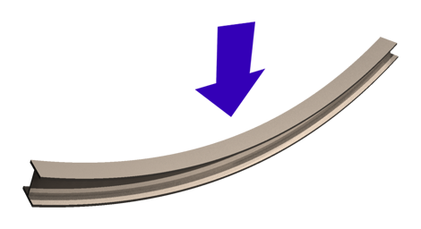
In applied mechanics, bending (also known as flexure) characterizes the behavior of a slender structural element subjected to an external load applied perpendicularly to a longitudinal axis of the element.

The structural element is assumed to be such that at least one of its dimensions is a small fraction, typically 1/10 or less, of the other two.[1] When the length is considerably longer than the width and the thickness, the element is called a beam. For example, a closet rod sagging under the weight of clothes on clothes hangers is an example of a beam experiencing bending. On the other hand, a shell is a structure of any geometric form where the length and the width are of the same order of magnitude but the thickness of the structure (known as the 'wall') is considerably smaller. A large diameter, but thin-walled, short tube supported at its ends and loaded laterally is an example of a shell experiencing bending.

In the absence of a qualifier, the term bending is ambiguous because bending can occur locally in all objects. Therefore, to make the usage of the term more precise, engineers refer to a specific object such as; the bending of rods,[2] the bending of beams,[1] the bending of plates,[3] the bending of shells[2] and so on.

Quasi-static bending of beams

[edit]

A beam deforms and stresses develop inside it when a transverse load is applied on it. In the quasi-static case, the amount of bending deflection and the stresses that develop are assumed not to change over time. In a horizontal beam supported at the ends and loaded downwards in the middle, the material at the over-side of the beam is compressed while the material at the underside is stretched. There are two forms of internal stresses caused by lateral loads:

  • Shear stress parallel to the lateral loading plus complementary shear stress on planes perpendicular to the load direction;
  • Direct compressive stress in the upper region of the beam, applicable mostly to cement concreted elements and,
  • Direct tensile stress, applicable to steel elements, and is at the lower region of the beam.

These last two forces form a couple or moment as they are equal in magnitude and opposite in direction. This bending moment resists the sagging deformation characteristic of a beam experiencing bending. The stress distribution in a beam can be predicted quite accurately when some simplifying assumptions are used.[1]

Euler–Bernoulli bending theory

[edit]
Element of a bent beam: the fibers form concentric arcs, the top fibers are compressed and bottom fibers stretched.
Bending moments in a beam

In the Euler–Bernoulli theory of slender beams, a major assumption is that 'plane sections remain plane'. In other words, any deformation due to shear across the section is not accounted for (no shear deformation). Also, this linear distribution is only applicable if the maximum stress is less than the yield stress of the material. For stresses that exceed yield, refer to article plastic bending. At yield, the maximum stress experienced in the section (at the furthest points from the neutral axis of the beam) is defined as the flexural strength.

Consider beams where the following are true:

  • The beam is originally straight and slender, and any taper is slight
  • The material is isotropic (or orthotropic), linear elastic, and homogeneous across any cross section (but not necessarily along its length)
  • Only small deflections are considered

In this case, the equation describing beam deflection () can be approximated as:

where the second derivative of its deflected shape with respect to is interpreted as its curvature, is the Young's modulus, is the area moment of inertia of the cross-section, and is the internal bending moment in the beam.

If, in addition, the beam is homogeneous along its length as well, and not tapered (i.e. constant cross section), and deflects under an applied transverse load , it can be shown that:[1]

This is the Euler–Bernoulli equation for beam bending.

After a solution for the displacement of the beam has been obtained, the bending moment () and shear force () in the beam can be calculated using the relations

Simple beam bending is often analyzed with the Euler–Bernoulli beam equation. The conditions for using simple bending theory are:[4]

  1. The beam is subject to pure bending. This means that the shear force is zero, and that no torsional or axial loads are present.
  2. The material is isotropic (or orthotropic) and homogeneous.
  3. The material obeys Hooke's law (it is linearly elastic and will not deform plastically).
  4. The beam is initially straight with a cross section that is constant throughout the beam length.
  5. The beam has an axis of symmetry in the plane of bending.
  6. The proportions of the beam are such that it would fail by bending rather than by crushing, wrinkling or sideways buckling.
  7. Cross-sections of the beam remain plane during bending.
Deflection of a beam deflected symmetrically and principle of superposition

Compressive and tensile forces develop in the direction of the beam axis under bending loads. These forces induce stresses on the beam. The maximum compressive stress is found at the uppermost edge of the beam while the maximum tensile stress is located at the lower edge of the beam. Since the stresses between these two opposing maxima vary linearly, there therefore exists a point on the linear path between them where there is no bending stress. The locus of these points is the neutral axis. Because of this area with no stress and the adjacent areas with low stress, using uniform cross section beams in bending is not a particularly efficient means of supporting a load as it does not use the full capacity of the beam until it is on the brink of collapse. Wide-flange beams (Ɪ-beams) and truss girders effectively address this inefficiency as they minimize the amount of material in this under-stressed region.

The classic formula for determining the bending stress in a beam under simple bending is:[5]

where

  • is the bending stress
  • – the moment about the neutral axis
  • – the perpendicular distance to the neutral axis
  • – the second moment of area about the neutral axis z.
  • - the Resistance Moment about the neutral axis z.

Extensions of Euler-Bernoulli beam bending theory

[edit]

Plastic bending

[edit]

The equation is valid only when the stress at the extreme fiber (i.e., the portion of the beam farthest from the neutral axis) is below the yield stress of the material from which it is constructed. At higher loadings the stress distribution becomes non-linear, and ductile materials will eventually enter a plastic hinge state where the magnitude of the stress is equal to the yield stress everywhere in the beam, with a discontinuity at the neutral axis where the stress changes from tensile to compressive. This plastic hinge state is typically used as a limit state in the design of steel structures.

Complex or asymmetrical bending

[edit]

The equation above is only valid if the cross-section is symmetrical. For homogeneous beams with asymmetrical sections, the maximum bending stress in the beam is given by

[6]

where are the coordinates of a point on the cross section at which the stress is to be determined as shown to the right, and are the bending moments about the y and z centroid axes, and are the second moments of area (distinct from moments of inertia) about the y and z axes, and is the product of moments of area. Using this equation it is possible to calculate the bending stress at any point on the beam cross section regardless of moment orientation or cross-sectional shape. Note that do not change from one point to another on the cross section.

Large bending deformation

[edit]

For large deformations of the body, the stress in the cross-section is calculated using an extended version of this formula. First the following assumptions must be made:

  1. Assumption of flat sections – before and after deformation the considered section of body remains flat (i.e., is not swirled).
  2. Shear and normal stresses in this section that are perpendicular to the normal vector of cross section have no influence on normal stresses that are parallel to this section.

Large bending considerations should be implemented when the bending radius is smaller than ten section heights h:

With those assumptions the stress in large bending is calculated as:

where

is the normal force
is the section area
is the bending moment
is the local bending radius (the radius of bending at the current section)
is the area moment of inertia along the x-axis, at the place (see Steiner's theorem)
is the position along y-axis on the section area in which the stress is calculated.

When bending radius approaches infinity and , the original formula is back:

.

Timoshenko bending theory

[edit]
Deformation of a Timoshenko beam. The normal rotates by an amount which is not equal to .

In 1921, Timoshenko improved upon the Euler–Bernoulli theory of beams by adding the effect of shear into the beam equation. The kinematic assumptions of the Timoshenko theory are:

  • normals to the axis of the beam remain straight after deformation
  • there is no change in beam thickness after deformation

However, normals to the axis are not required to remain perpendicular to the axis after deformation.

The equation for the quasistatic bending of a linear elastic, isotropic, homogeneous beam of constant cross-section beam under these assumptions is[7]

where is the area moment of inertia of the cross-section, is the cross-sectional area, is the shear modulus, is a shear correction factor, and is an applied transverse load. For materials with Poisson's ratios () close to 0.3, the shear correction factor for a rectangular cross-section is approximately

The rotation () of the normal is described by the equation

The bending moment () and the shear force () are given by

Beams on elastic foundations

[edit]

According to Euler–Bernoulli, Timoshenko or other bending theories, the beams on elastic foundations can be explained. In some applications such as rail tracks, foundation of buildings and machines, ships on water, roots of plants etc., the beam subjected to loads is supported on continuous elastic foundations (i.e. the continuous reactions due to external loading is distributed along the length of the beam)[8][9][10][11]

Car crossing a bridge (Beam partially supported on elastic foundation, Bending moment distribution)

Dynamic bending of beams

[edit]

The dynamic bending of beams,[12] also known as flexural vibrations of beams, was first investigated by Daniel Bernoulli in the late 18th century. Bernoulli's equation of motion of a vibrating beam tended to overestimate the natural frequencies of beams and was improved marginally by Rayleigh in 1877 by the addition of a mid-plane rotation. In 1921 Stephen Timoshenko improved the theory further by incorporating the effect of shear on the dynamic response of bending beams. This allowed the theory to be used for problems involving high frequencies of vibration where the dynamic Euler–Bernoulli theory is inadequate. The Euler-Bernoulli and Timoshenko theories for the dynamic bending of beams continue to be used widely by engineers.

Euler–Bernoulli theory

[edit]

The Euler–Bernoulli equation for the dynamic bending of slender, isotropic, homogeneous beams of constant cross-section under an applied transverse load is[7]

where is the Young's modulus, is the area moment of inertia of the cross-section, is the deflection of the neutral axis of the beam, and is mass per unit length of the beam.

Free vibrations

[edit]

For the situation where there is no transverse load on the beam, the bending equation takes the form

Free, harmonic vibrations of the beam can then be expressed as

and the bending equation can be written as

The general solution of the above equation is

where are constants and

The mode shapes of a cantilevered Ɪ-beam
1st lateral bending
1st torsional
1st vertical bending
2nd lateral bending
2nd torsional
2nd vertical bending

Timoshenko–Rayleigh theory

[edit]

In 1877, Rayleigh proposed an improvement to the dynamic Euler–Bernoulli beam theory by including the effect of rotational inertia of the cross-section of the beam. Timoshenko improved upon that theory in 1922 by adding the effect of shear into the beam equation. Shear deformations of the normal to the mid-surface of the beam are allowed in the Timoshenko–Rayleigh theory.

The equation for the bending of a linear elastic, isotropic, homogeneous beam of constant cross-section under these assumptions is[7][13]

where is the polar moment of inertia of the cross-section, is the mass per unit length of the beam, is the density of the beam, is the cross-sectional area, is the shear modulus, and is a shear correction factor. For materials with Poisson's ratios () close to 0.3, the shear correction factor are approximately

Free vibrations

[edit]

For free, harmonic vibrations the Timoshenko–Rayleigh equations take the form

This equation can be solved by noting that all the derivatives of must have the same form to cancel out and hence as solution of the form may be expected. This observation leads to the characteristic equation

The solutions of this quartic equation are

where

The general solution of the Timoshenko-Rayleigh beam equation for free vibrations can then be written as

Quasistatic bending of plates

[edit]
Deformation of a thin plate highlighting the displacement, the mid-surface (red) and the normal to the mid-surface (blue)

The defining feature of beams is that one of the dimensions is much larger than the other two. A structure is called a plate when it is flat and one of its dimensions is much smaller than the other two. There are several theories that attempt to describe the deformation and stress in a plate under applied loads two of which have been used widely. These are

  • the Kirchhoff–Love theory of plates (also called classical plate theory)
  • the Mindlin–Reissner plate theory (also called the first-order shear theory of plates)

Kirchhoff–Love theory of plates

[edit]

The assumptions of Kirchhoff–Love theory are

  • straight lines normal to the mid-surface remain straight after deformation
  • straight lines normal to the mid-surface remain normal to the mid-surface after deformation
  • the thickness of the plate does not change during a deformation.

These assumptions imply that

where is the displacement of a point in the plate and is the displacement of the mid-surface.

The strain-displacement relations are

The equilibrium equations are

where is an applied load normal to the surface of the plate.

In terms of displacements, the equilibrium equations for an isotropic, linear elastic plate in the absence of external load can be written as

In direct tensor notation,

Mindlin–Reissner theory of plates

[edit]

The special assumption of this theory is that normals to the mid-surface remain straight and inextensible but not necessarily normal to the mid-surface after deformation. The displacements of the plate are given by

where are the rotations of the normal.

The strain-displacement relations that result from these assumptions are

where is a shear correction factor.

The equilibrium equations are

where

Dynamic bending of plates

[edit]

Dynamics of thin Kirchhoff plates

[edit]

The dynamic theory of plates determines the propagation of waves in the plates, and the study of standing waves and vibration modes. The equations that govern the dynamic bending of Kirchhoff plates are

where, for a plate with density ,

and

The figures below show some vibrational modes of a circular plate.

See also

[edit]

References

[edit]
[edit]
Revisions and contributorsEdit on WikipediaRead on Wikipedia
from Grokipedia
Bending is a fundamental deformation mode in where a beam or slender undergoes due to the application of a , a couple of forces that induces internal normal stresses varying across the cross-section. This process, also known as , occurs when transverse loads are applied perpendicular to the element's longitudinal axis, causing one side to experience tension and the opposite side compression, with zero stress along the at the . In contexts, bending is critical for analyzing the strength and stability of beams, columns, and other load-bearing components in buildings, bridges, and machinery. The , defined as the resultant moment of forces about a point on the beam's cross-section, quantifies the intensity of bending and is determined through shear and moment diagrams that illustrate its variation along the structure's length. Shear forces, which accompany bending moments, contribute to transverse deformation but are secondary to the primary effect. Key assumptions in include linear elastic material behavior, small deformations, and plane sections remaining plane after bending, enabling the use of the Euler-Bernoulli for most practical analyses. The normal stress due to bending is calculated using the flexure formula σ=MyI\sigma = \frac{M y}{I}, where σ\sigma is the stress, MM is the bending moment, yy is the distance from the neutral axis, and II is the second moment of area (moment of inertia) of the cross-section, which measures the section's resistance to bending. This stress distribution is linear, peaking at the outermost fibers, and determines the maximum allowable load before yielding or failure. In design, engineers select materials and cross-sectional shapes—such as I-beams with high II values—to optimize resistance to bending while minimizing weight. Advanced considerations include combined bending with axial loads or torsion, and nonlinear effects in large deformations or plastic regimes.

Fundamentals of Bending

Definition and Basic Mechanics

Bending is the deformation mode in which slender structural elements, such as beams, undergo when subjected to transverse loads that generate internal bending moments opposing the applied forces. This arises from the of cross-sections to the beam's longitudinal axis, assuming small deformations where plane sections remain plane. The phenomenon is fundamental in , enabling the analysis of load-bearing capacity in applications like bridges and components. The kinematic description of bending involves key geometric elements: the , which passes through the of the cross-section and experiences no longitudinal strain; the ρ, which quantifies the beam's ; and the linear variation of normal strain ε_x with distance y from the neutral axis, given by ϵx=yρ,\epsilon_x = -\frac{y}{\rho}, where the negative sign indicates compressive strain above the neutral axis for positive curvature (concave upward). This relation derives from the of deformation, where fibers above the neutral axis shorten and those below elongate proportionally to their distance from it. From static equilibrium considerations, the internal forces in a beam include the shear force V, which resists transverse loads, and the bending moment M, which resists rotation. These are related by the differential equation dMdx=V,\frac{dM}{dx} = V, obtained by summing moments about a differential element along the beam's length x, ensuring force and moment balance under quasi-static conditions. Early insights into bending mechanics trace back to Galileo Galilei, who in 1638 published observations on the resistance of cantilever beams to transverse loads in his Dialogues Concerning Two New Sciences, modeling the beam as a lever and estimating its breaking strength based on the moment arm. To illustrate moment distribution, consider a simple cantilever beam of length L fixed at x=0 and loaded by a point force P downward at the free end x=L; the shear force V is constant at -P along the length, while the bending moment M(x) = -P(L - x) varies linearly from 0 at the free end to -PL at the fixed support, highlighting the maximum moment concentration at the clamped end.

Stress and Strain Distribution

In the analysis of bending, the distribution of normal stress and strain across a beam's cross-section is derived under the assumptions of small deformations, where plane sections to the beam axis remain plane after bending, and the is homogeneous, isotropic, and behaves linearly elastic according to with predominant uniaxial stress. These conditions ensure that longitudinal strains vary linearly with the distance from the , transitioning from compression above the axis to tension below it. Applying Hooke's law, σx=Eϵx\sigma_x = E \epsilon_x, the normal stress σx\sigma_x at a point distance yy from the is given by σx=MyI,\sigma_x = -\frac{M y}{I}, where MM is the internal , II is the second moment of area () of the cross-section about the , and the negative sign indicates compression for positive MM and yy. This linear stress profile arises from the equilibrium of moments and the linear strain distribution, with maximum compressive and tensile stresses occurring at the extreme fibers farthest from the . The corresponding axial strain ϵx\epsilon_x follows directly from Hooke's law as ϵx=σxE=MyEI,\epsilon_x = \frac{\sigma_x}{E} = -\frac{M y}{E I}, exhibiting a linear variation across the cross-section: zero at the , negative (compressive) in the region above it, and positive (tensile) below it for typical sagging bending. This strain profile confirms the kinematic assumption of plane sections remaining plane, with the magnitude of strain proportional to yy. In addition to normal stresses, transverse shear stresses arise due to the shear force VV acting parallel to the cross-section. The average shear stress is approximated as τavg=V/A\tau_\mathrm{avg} = V / A, where AA is the cross-sectional area, providing a uniform distribution for preliminary . However, the actual distribution is parabolic, varying from zero at the top and bottom surfaces to a maximum at the , as derived from equilibrium considerations of horizontal shear flows in beam elements. To illustrate, consider a rectangular beam of width bb and height hh subjected to a uniform MM. The is I=bh3/12I = b h^3 / 12, and the maximum distance from the is ymax=h/2y_\mathrm{max} = h/2. The maximum normal stress at the outer fibers is then σmax=M(h/2)bh3/12=6Mbh2.\sigma_\mathrm{max} = \frac{M (h/2)}{b h^3 / 12} = \frac{6M}{b h^2}. For example, if b=0.1b = 0.1 m, h=0.2h = 0.2 m, and M=1000M = 1000 Nm, then σmax=1.5\sigma_\mathrm{max} = 1.5 MPa, representing the peak tensile or .

Quasi-Static Bending of Beams

Euler-Bernoulli Beam Theory

The Euler-Bernoulli beam theory provides a foundational framework for analyzing the quasi-static bending of slender beams, assuming small deflections and neglecting shear deformation effects. Developed in the mid-18th century, the theory integrates contributions from Leonhard Euler's work on elastic curves in 1744 and Daniel Bernoulli's earlier insights into beam resistance, establishing the relationship between applied moments and beam curvature. This classical approach models beams as one-dimensional elements where the primary deformation arises from bending, enabling straightforward calculations of deflections and internal forces under transverse loads. Central to the theory are kinematic assumptions that plane cross-sections originally perpendicular to the beam's neutral axis remain plane and perpendicular after deformation, implying no distortion in the cross-section and zero transverse shear strain. The beam material is assumed to be linearly elastic, homogeneous, and isotropic, with small deflections ensuring geometric linearity. These hypotheses lead to the core relation linking curvature κ\kappa to the bending moment MM, where κ=1/ρd2v/dx2=M/(EI)\kappa = 1/\rho \approx d^2 v / dx^2 = -M / (EI), with v(x)v(x) denoting transverse deflection, EE the modulus of elasticity, and II the second moment of area about the neutral axis. Integrating the equilibrium equations for a beam under distributed load q(x)q(x) yields the fourth-order boundary value problem EId4v/dx4=q(x)EI \, d^4 v / dx^4 = q(x) for constant flexural rigidity EIEI, solved subject to appropriate boundary conditions such as clamped, free, or supported ends. Analytical solutions for common loading and support configurations illustrate the theory's utility. For a simply supported beam of length LL under uniform distributed load qq, the deflection is given by v(x)=qx24EI(L32Lx2+x3),v(x) = \frac{q x}{24 EI} (L^3 - 2 L x^2 + x^3), achieving maximum deflection v(L/2)=5qL4/(384EI)v(L/2) = 5 q L^4 / (384 EI) at midspan. This expression derives from integrating the governing equation twice for shear and moment, then applying boundary conditions v(0)=v(L)=0v(0) = v(L) = 0 and zero moments at ends. While effective for slender beams where the length-to-depth ratio exceeds approximately 10, the theory exhibits limitations for shorter or thicker beams, overpredicting stiffness by ignoring shear deformation contributions that become significant in such cases.

Timoshenko Beam Theory

The Timoshenko beam theory extends the Euler-Bernoulli beam theory by incorporating transverse shear deformation, providing a more accurate model for the quasi-static bending of moderately thick beams where shear effects cannot be neglected. Developed in the early , this theory relaxes the assumption that plane cross-sections remain perpendicular to the after deformation, allowing for a shear angle between the cross-section and the beam's longitudinal axis. While rotary is also included in the full formulation, the quasi-static case focuses primarily on shear deformation to capture increased deflections in beams with significant depth-to-span ratios. The kinematics of the Timoshenko beam are defined by the transverse deflection v(x)v(x) and the rotation of the cross-section ψ(x)\psi(x), leading to the shear strain γ=dvdxψ\gamma = \frac{dv}{dx} - \psi. The constitutive relations are given by the bending moment M=EIdψdxM = EI \frac{d\psi}{dx} and the shear force V=κGAγV = \kappa GA \gamma, where EE is the Young's modulus, II is the second moment of area, GG is the shear modulus, AA is the cross-sectional area, and κ\kappa is the shear correction factor that accounts for the non-uniform shear stress distribution across the section (e.g., κ=5/6\kappa = 5/6 for rectangular sections). Equilibrium equations for a beam under distributed transverse load q(x)q(x) yield dVdx=q\frac{dV}{dx} = -q and dMdx=V\frac{dM}{dx} = V, resulting in the coupled second-order differential equations: κGA(d2vdx2dψdx)+q=0,\kappa GA \left( \frac{d^2 v}{dx^2} - \frac{d\psi}{dx} \right) + q = 0, EId2ψdx2+κGA(dvdxψ)=0.EI \frac{d^2 \psi}{dx^2} + \kappa GA \left( \frac{dv}{dx} - \psi \right) = 0. These equations must be solved simultaneously with appropriate boundary conditions, such as for a simply supported beam where v(0)=v(L)=0v(0) = v(L) = 0 and M(0)=M(L)=0M(0) = M(L) = 0. In the limit of slender beams (large LL relative to depth), the theory reduces to the Euler-Bernoulli model by setting ψ=dv/dx\psi = dv/dx. For a simply supported beam of LL under uniform load qq, the maximum deflection at the midspan includes a flexural component identical to the Euler-Bernoulli prediction and an additional shear term vshear=qL28κGAv_{\text{shear}} = \frac{q L^2}{8 \kappa G A}. The total deflection is thus larger than the Euler-Bernoulli value by the approximate factor 1+12EIκGAL21 + \frac{12 EI}{\kappa G A L^2}, highlighting the shear correction's significance for beams where this factor exceeds 0.1 (e.g., depth-to-span ratios greater than about 1:10). This increased deflection prediction is crucial for applications involving composite or sandwich beams, where low transverse shear in the core or interfaces amplifies deformation beyond Euler-Bernoulli estimates.

Extensions for Nonlinear and Complex Cases

In the realm of quasi-static beam bending, extensions beyond linear elastic theory are essential for capturing material nonlinearity, geometric nonlinearity, and loading asymmetries that arise in practical scenarios. Plastic bending addresses the behavior of beams under elastic-perfectly plastic materials, where yielding initiates at the outer fibers when the maximum stress reaches the yield stress σy=My/I\sigma_y = M y / I, with MM as the , yy the distance from the to the outer fiber, and II the . For a rectangular cross-section of width bb and hh, the elastic limit moment is Me=σybh2/6M_e = \sigma_y b h^2 / 6, marking the onset of plasticity. As the moment increases, an elastic core persists while outer regions yield, leading to a moment-curvature relation M=σyb(3h24c2)/12M = \sigma_y b (3 h^2 - 4 c^2) / 12, where cc is the half- of the elastic core; the fully plastic moment, representing collapse, is Mp=σybh2/4M_p = \sigma_y b h^2 / 4, providing 1.5 times the elastic capacity for rectangular sections. Geometric nonlinearity becomes prominent in large deformation regimes, where moderate rotations invalidate small-angle approximations. The exact curvature is defined as κ=dθ/ds\kappa = d\theta / ds, with θ\theta the rotation angle and ss the arc length along the beam centerline, contrasting the linear κd2w/dx2\kappa \approx d^2 w / dx^2. For moderate deflections (θ10\theta \leq 10^\circ), von Kármán strains incorporate nonlinear axial effects: ϵx=du/dx+12(dw/dx)2\epsilon_x = du/dx + \frac{1}{2} (dw/dx)^2, coupling bending with axial stretching and altering equilibrium to d2M/dx2+Nd2w/dx2+q=0-d^2 M / dx^2 + N d^2 w / dx^2 + q = 0, where NN is the axial force and qq the distributed load. This framework is crucial for beams with axial constraints, enabling accurate prediction of stiffening due to membrane action. Asymmetrical bending occurs under biaxial moments MyM_y and MzM_z, particularly for unsymmetric cross-sections, causing the to shift from principal axes. The product of IyzI_{yz} introduces , with the normal stress given by σx=(MzIyMyIyz)y+(MyIzMzIyz)zIyIzIyz2\sigma_x = \frac{(M_z I_y - M_y I_{yz}) y + (M_y I_z - M_z I_{yz}) z}{I_y I_z - I_{yz}^2}, where yy and zz are coordinates from the , and IyI_y, IzI_z are moments of about the yy and zz axes. This formulation accounts for the inclined , preventing erroneous stress predictions in non-orthogonal loading. For complex cases involving thin-walled beams, combined bending and torsion demands specialized theories to handle warping and distortion. Vlasov's theory, introduced in and refined in his monograph, extends classical beam models by incorporating a warping function and bimoment to capture nonuniform torsion in open cross-sections, yielding coupled differential equations for bending-torsion interaction under eccentric or skewed loads. These extensions are vital for stability analysis in slender structures. Post-World War II developments in nonlinear and complex bending theories were heavily influenced by the demands of high-speed aircraft design, emphasizing plasticity and large deformations to optimize lightweight aluminum and composite spars against and . Seminal works, such as Bruhn's 1949 manual (expanded in 1965), integrated these extensions into practical analysis, prioritizing shape factors and limit states for wing and beams.

Beams on Elastic Foundations

Winkler Foundation Model

The Winkler foundation model conceptualizes the supporting medium beneath a beam as a dense array of discrete, mutually independent linear elastic springs, each reacting proportionally to the local vertical deflection of the beam. Introduced by Emil Winkler in his 1867 treatise on elasticity and strength, this approach idealizes the foundation reaction pressure p(x)p(x) at any point along the beam as p(x)=kv(x)p(x) = k v(x), where v(x)v(x) is the beam deflection and kk is the foundation modulus (with units of force per unit length per unit deflection for a beam of unit width). This linear relationship assumes that deflections at adjacent points do not influence one another, effectively neglecting shear resistance within the foundation material. When incorporated into the Euler-Bernoulli beam equation, the model yields the governing differential equation for quasi-static bending: EId4vdx4+kv(x)=q(x),EI \frac{d^4 v}{dx^4} + k v(x) = q(x), where EIEI is the beam's flexural rigidity and q(x)q(x) is the applied distributed load per unit length. This fourth-order ordinary differential equation characterizes the beam's response, with solutions decaying exponentially away from load application regions. A key parameter is the characteristic length λ=(k4EI)1/4\lambda = \left( \frac{k}{4 EI} \right)^{1/4}, which defines the distance over which significant deflections occur; beams much longer than 1/λ1/\lambda behave as effectively infinite, while shorter ones exhibit boundary effects. Analytical solutions are obtained by solving the homogeneous equation EIv+kv=0EI v'''' + k v = 0, yielding roots that lead to oscillatory-decay functions of the form eλx(cosλx+sinλx)e^{-\lambda x} (\cos \lambda x + \sin \lambda x) and eλxcosλxe^{-\lambda x} \cos \lambda x. For an infinite beam under a concentrated point load PP at x=0x = 0, the deflection takes the closed-form expression v(x)=P8EIλ3eλx(cosλx+sinλx),v(x) = \frac{P}{8 EI \lambda^3} e^{-\lambda |x|} \left( \cos \lambda |x| + \sin \lambda |x| \right), which satisfies the governing equation and ensures continuity of deflection, slope, moment, and shear at the load point. At x=0x = 0, the maximum deflection simplifies to v(0)=P8EIλ3v(0) = \frac{P}{8 EI \lambda^3}, highlighting the inverse dependence on foundation stiffness through λ\lambda. This solution, derived systematically in classical treatments, illustrates the localized nature of deformations under the Winkler assumption, with deflections approaching zero as x|x| increases beyond several multiples of 1/λ1/\lambda. The model's primary assumptions—independent spring responses and unilateral contact (no tension in the foundation)—make it computationally tractable for preliminary but limit its accuracy in scenarios involving stiff or cohesive soils, where lateral interactions propagate stresses beyond local deflections. Despite these constraints, it remains foundational for applications such as railroad track analysis, where and are approximated as Winkler springs to assess rail deflections under loads, and mat foundations for structures, enabling simplified evaluation of settlement and bending in spread footings. For denser soils, the lack of inter-spring can overestimate settlements, prompting the development of continuum-based alternatives.

More Advanced Foundation Models

More advanced foundation models extend the Winkler approach by incorporating continuum effects such as shear deformation and in the supporting medium, leading to more realistic representations of for beams under quasi-static bending. These two-parameter models address limitations in the Winkler foundation, such as the unrealistic of support points, by introducing a second that accounts for lateral continuity and shear resistance. The Pasternak model, proposed in 1954, augments the Winkler springs with a shear layer that connects adjacent points, modeling the foundation reaction as p=kvGfd2vdx2p = k v - G_f \frac{d^2 v}{dx^2}, where kk is the Winkler modulus, vv is the beam deflection, and GfG_f is the of the foundation. This formulation captures the shearing effect in soils, preventing the discontinuous deflection profiles characteristic of the Winkler model. For an Euler-Bernoulli beam on a Pasternak foundation, the governing becomes EId4vdx4Gfd2vdx2+kv=q(x),EI \frac{d^4 v}{dx^4} - G_f \frac{d^2 v}{dx^2} + k v = q(x), where EIEI is the beam and q(x)q(x) is the applied load. Analytical solutions for infinite or semi-infinite beams are often obtained using Fourier transforms, which decompose the problem into harmonic components for efficient computation of deflection and moment distributions. Other two-parameter models, such as those developed by Kerr in 1964 and Vlasov and Leontiev in 1966, further refine the representation by incorporating soil compressibility and inter-layer interactions. The Kerr model treats the foundation as multiple spring layers with shear connections, providing a versatile framework for viscoelastic or heterogeneous soils. In contrast, the Vlasov model assumes a compressible where the reaction modulus varies with depth, effectively modeling the foundation as a continuum with reduced away from the surface. These approaches yield deflection profiles that are smoother and exhibit reduced oscillations compared to the Winkler model, particularly under concentrated loads, as the shear and compression parameters distribute reactions more uniformly across the beam length. Post-1960s developments have integrated these models into finite element methods, enabling analysis of beams on uneven or spatially varying foundations where parameters like kk and GfG_f are functions of position to reflect heterogeneous soils. This numerical approach facilitates practical applications in , such as pipeline or mat foundation design, by allowing for irregular geometries and material properties without relying on simplified analytical assumptions.

Dynamic Bending of Beams

Free Vibrations in Euler-Bernoulli Beams

The free vibrations of slender beams are analyzed using Euler-Bernoulli beam theory, which assumes that plane sections remain plane and perpendicular to the after deformation, neglecting shear deformation and rotary . This approach is suitable for high-frequency modes in long, thin beams where bending dominates. The governing equation of motion for transverse vibrations without external loads is derived from Newton's second law applied to beam elements, yielding EI4vx4+ρA2vt2=0,EI \frac{\partial^4 v}{\partial x^4} + \rho A \frac{\partial^2 v}{\partial t^2} = 0, where EE is the Young's modulus, II is the second moment of area, ρ\rho is the material density, AA is the cross-sectional area, v(x,t)v(x,t) is the transverse displacement, xx is the position along the beam length, and tt is time. To solve this partial differential equation, the method of separation of variables is employed, assuming a solution of the form v(x,t)=ϕ(x)sin(ωt+θ)v(x,t) = \phi(x) \sin(\omega t + \theta), where ϕ(x)\phi(x) is the spatial mode shape and ω\omega is the natural frequency. Substituting this into the equation of motion results in the ordinary differential equation EId4ϕdx4ρAω2ϕ=0,EI \frac{d^4 \phi}{dx^4} - \rho A \omega^2 \phi = 0, with the general solution ϕ(x)=Asin(βx)+Bcos(βx)+Csinh(βx)+Dcosh(βx)\phi(x) = A \sin(\beta x) + B \cos(\beta x) + C \sinh(\beta x) + D \cosh(\beta x), where β4=ρAω2/EI\beta^4 = \rho A \omega^2 / EI. The constants A,B,C,DA, B, C, D are determined by applying boundary conditions specific to the beam supports. For a pinned-pinned beam of length LL, the boundary conditions are ϕ(0)=ϕ(L)=0\phi(0) = \phi(L) = 0 and ϕ(0)=ϕ(L)=0\phi''(0) = \phi''(L) = 0. These yield the mode shapes ϕn(x)=sin(nπxL)\phi_n(x) = \sin\left(\frac{n \pi x}{L}\right) for n=1,2,3,n = 1, 2, 3, \dots, and the corresponding natural frequencies ωn=(nπL)2EIρA\omega_n = \left(\frac{n \pi}{L}\right)^2 \sqrt{\frac{EI}{\rho A}}
Add your contribution
Related Hubs
User Avatar
No comments yet.