


Community hub
Wikipedia
Integration by reduction formulae
View on Wikipedia| Part of a series of articles about |
| Calculus |
|---|
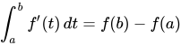
In integral calculus, integration by reduction formulae is a method relying on recurrence relations. It is used when an expression containing an integer parameter, usually in the form of powers of elementary functions, or products of transcendental functions and polynomials of arbitrary degree, cannot be integrated directly. Using other methods of integration a reduction formula can be set up to obtain the integral of the same or similar expression with a lower integer parameter, progressively simplifying the integral until it can be evaluated. [1] This method of integration is one of the earliest used.[citation needed]
How to find the reduction formula
[edit]The reduction formula can be derived using any of the common methods of integration, like integration by substitution, integration by parts, integration by trigonometric substitution, integration by partial fractions, etc. The main idea is to express an integral involving an integer parameter (e.g. power) of a function, represented by In, in terms of an integral that involves a lower value of the parameter (lower power) of that function, for example In-1 or In-2. This makes the reduction formula a type of recurrence relation. In other words, the reduction formula expresses the integral
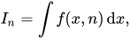
in terms of
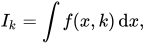
where

Reference works contain the general forms for recursive integration (see, for example Gradshteyn and Ryzhik).
How to compute the integral
[edit]To compute the integral, we set n to its value and use the reduction formula to express it in terms of the (n – 1) or (n – 2) integral. The lower index integral can be used to calculate the higher index ones; the process is continued repeatedly until we reach a point where the function to be integrated can be computed, usually when its index is 0 or 1. Then we back-substitute the previous results until we have computed In. [2]
Examples
[edit]Below are examples of the procedure.
Cosine integral
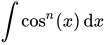
[edit]Typically, integrals like
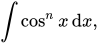
can be evaluated by a reduction formula.

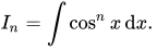
Start by setting:
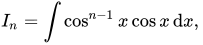
Now re-write as:
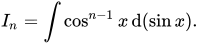
Integrating by this substitution:

Now integrating by parts:
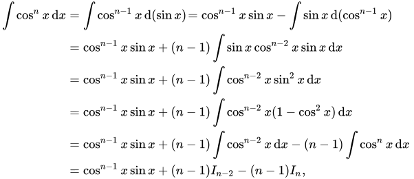
solving for In:



so the reduction formula is:

To supplement the example, the above can be used to evaluate the integral for (say) n = 5;
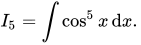
Calculating lower indices:


back-substituting:


![{\displaystyle I_{5}\ ={\frac {1}{5}}\cos ^{4}x\sin x+{\frac {4}{5}}\left[{\frac {1}{3}}\cos ^{2}x\sin x+{\frac {2}{3}}\sin x\right]+C,\,}](https://wikimedia.org/api/rest_v1/media/math/render/svg/7803bf2d86071f40537d4590e76ab498354b7c7f)
where C is a constant.
Exponential integral
[edit]Another typical example is:

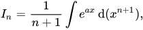
Start by setting:
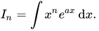
Integrating by substitution:
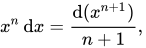
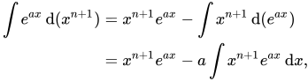
Now integrating by parts:

shifting indices back by 1 (so n + 1 → n, n → n – 1):

solving for In:
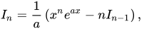
so the reduction formula is:

An alternative way in which the derivation could be done starts by substituting .

Integration by substitution:
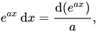
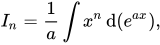
Now integrating by parts:
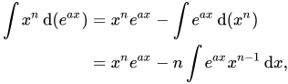
which gives the reduction formula when substituting back:
which is equivalent to:
Another alternative way in which the derivation could be done by integrating by parts:
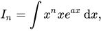

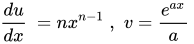


Remember:
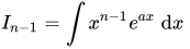
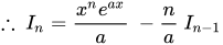
which gives the reduction formula when substituting back:
which is equivalent to:
Tables of integral reduction formulas
[edit]Rational functions
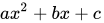
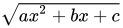
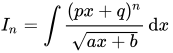
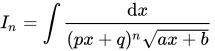
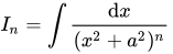
[edit]The following integrals[3] contain:
- Factors of the linear radical
- Linear factors and the linear radical
- Quadratic factors
- Quadratic factors , for
- Quadratic factors , for
- (Irreducible) quadratic factors
- Radicals of irreducible quadratic factors


| Integral | Reduction formula |
|---|---|
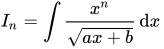

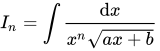

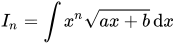

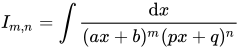
![{\displaystyle I_{m,n}={\begin{cases}-{\frac {1}{(n-1)(bp-aq)}}\left[{\frac {1}{(ax+b)^{m-1}(px+q)^{n-1}}}+a(m+n-2)I_{m,n-1}\right]\\{\frac {1}{(m-1)(bp-aq)}}\left[{\frac {1}{(ax+b)^{m-1}(px+q)^{n-1}}}+p(m+n-2)I_{m-1,n}\right]\end{cases}}\,\!}](https://wikimedia.org/api/rest_v1/media/math/render/svg/22e62922721540ee6636beadc5183d305fa0a98b)
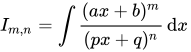
![{\displaystyle I_{m,n}={\begin{cases}-{\frac {1}{(n-1)(bp-aq)}}\left[{\frac {(ax+b)^{m+1}}{(px+q)^{n-1}}}+a(n-m-2)I_{m,n-1}\right]\\-{\frac {1}{(n-m-1)p}}\left[{\frac {(ax+b)^{m}}{(px+q)^{n-1}}}+m(bp-aq)I_{m-1,n}\right]\\-{\frac {1}{(n-1)p}}\left[{\frac {(ax+b)^{m}}{(px+q)^{n-1}}}-amI_{m-1,n-1}\right]\end{cases}}\,\!}](https://wikimedia.org/api/rest_v1/media/math/render/svg/18cf63aea753eb3517e589623b4728e1545c012b)
| Integral | Reduction formula |
|---|---|
|
| |
|
|




| Integral | Reduction formula |
|---|---|

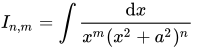

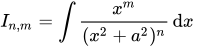

| Integral | Reduction formula |
|---|---|
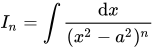

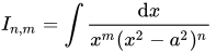

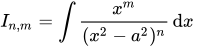

| Integral | Reduction formula |
|---|---|
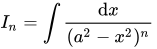

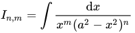

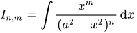

| Integral | Reduction formula |
|---|---|
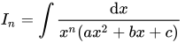



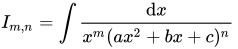

| Integral | Reduction formula |
|---|---|


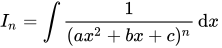

note that by the laws of indices:

Transcendental functions
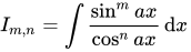
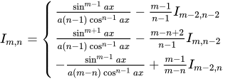
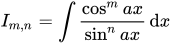
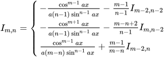
[edit]The following integrals[4] contain:
- Factors of sine
- Factors of cosine
- Factors of sine and cosine products and quotients
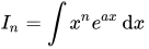
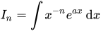
- Products/quotients of exponential factors and powers of x
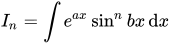
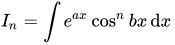
- Products of exponential and sine/cosine factors
| Integral | Reduction formula |
|---|---|
|
|
the formulae can be combined to obtain separate equations in In:
and Jn:
|
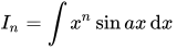

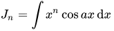

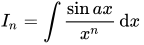




![{\displaystyle I_{n}=-{\frac {\sin {ax}}{(n-1)x^{n-1}}}-{\frac {a}{n-1}}\left[{\frac {\cos {ax}}{(n-2)x^{n-2}}}+{\frac {a}{n-2}}I_{n-2}\right]\,\!}](https://wikimedia.org/api/rest_v1/media/math/render/svg/c59ab79c10f4eed2620c496fac8b476174a84477)


![{\displaystyle J_{n}=-{\frac {\cos {ax}}{(n-1)x^{n-1}}}-{\frac {a}{n-1}}\left[-{\frac {\sin {ax}}{(n-2)x^{n-2}}}+{\frac {a}{n-2}}J_{n-2}\right]\,\!}](https://wikimedia.org/api/rest_v1/media/math/render/svg/cf2ed60b99d5d7b4dfa736c3627c68021c847b44)

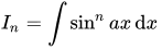

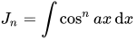

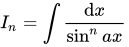

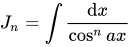

| Integral | Reduction formula |
|---|---|

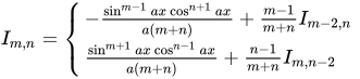
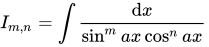

| Integral | Reduction formula |
|---|---|
|
|
|
|
|
|






References
[edit]- ^ Mathematical methods for physics and engineering, K.F. Riley, M.P. Hobson, S.J. Bence, Cambridge University Press, 2010, ISBN 978-0-521-86153-3
- ^ Further Elementary Analysis, R.I. Porter, G. Bell & Sons Ltd, 1978, ISBN 0-7135-1594-5
- ^ http://www.sosmath.com/tables/tables.html -> Indefinite integrals list
- ^ http://www.sosmath.com/tables/tables.html -> Indefinite integrals list
Bibliography
[edit]
- Anton, Bivens, Davis, Calculus, 7th edition.
Grokipedia
Integration by reduction formulae
View on GrokipediaBasic Concepts
Definition of Reduction Formulae
Reduction formulae in integral calculus are recursive relations that express an integral involving a parameter, typically an integer $ n $, in terms of an integral with a reduced value of that parameter, such as $ n-2 $ or $ n-1 $. These formulae take the general form $ I_n = f(n) I_{n-k} + g(n) $, where $ I_n = \int x^n h(x) , dx $ or a similar parameterized integral, and $ f(n) $, $ g(n) $, and $ k $ are functions or constants depending on the specific case, enabling the computation of higher-order integrals by relating them to simpler, lower-order ones.[4][5] The primary purpose of reduction formulae is to evaluate definite or indefinite integrals that do not yield to direct methods for finding antiderivatives, particularly those involving powers of trigonometric, exponential, or polynomial functions, or products thereof. By iteratively applying the recursive relation, the integral is reduced until it reaches a base case that can be computed explicitly, such as $ I_0 $ or $ I_1 $, which often involves elementary functions. Key properties include their recursive structure, which ensures a finite number of steps for integer parameters, the necessity of establishing base cases for termination, and considerations of convergence or validity for specific ranges of $ n $, such as positive even or odd integers.[4][5] These formulae originated in 18th- and 19th-century calculus texts as tools for handling integrals that were non-elementary or cumbersome, building on foundational integration techniques like integration by parts.[6]Connection to Integration by Parts
Integration by parts is a fundamental integration technique derived from the product rule of differentiation, expressed by the formulaDeriving Reduction Formulae
Standard Derivation via Integration by Parts
The standard derivation of reduction formulae employs integration by parts, a technique rooted in the product rule for differentiation, to express an integral involving a power in terms of a similar integral with a reduced power, typically .[7] To derive such a formula generally, begin by defining the integral , where and are suitable functions. Apply integration by parts by setting and , so that and . The formula then yields , which simplifies to an expression relating to after algebraic manipulation, often using identities like if applicable.[3] A prototypical example is the derivation for , where . Set and , yielding and . Substituting into the integration by parts formula gives:Derivation Using Differentiation Under the Integral Sign
Differentiation under the integral sign provides an alternative approach to deriving reduction formulae by introducing a parameter into the integrand and applying the Leibniz integral rule, which allows interchanging differentiation and integration under suitable conditions. Consider an integral defined as a function of a parameter , . Differentiating both sides with respect to yields , assuming the operations can be interchanged, which holds for continuous functions and appropriate domains. Integrating back with respect to or evaluating at specific values relates to simpler forms, often leading to recursive relations that reduce the complexity of the original integral.[11] A classic example arises in deriving the reduction formula for the Gamma function, defined as for positive integers . Introduce the parameter to form . Differentiating both sides times with respect to gives . Setting yields the relation , which serves as the reduction formula connecting to the lower-order . This method extends naturally to non-integer cases for the full Gamma function.[11][12] This technique offers advantages over direct methods like integration by parts, particularly for definite integrals where boundary terms vanish, avoiding complications from indefinite forms, and producing cleaner recursive relations for special functions such as the Gamma or Beta functions. It is especially useful for integrals involving parameters, such as the exponential decay in where , or trigonometric integrals expressed via complex exponentials, like through Euler's formula relating sines to imaginaries of exponentials.[11][12] The method was popularized by Gottfried Wilhelm Leibniz in a 1697 letter to Johann Bernoulli, where it appeared as a tool for evaluating parametric integrals, and later became central to the theory of special functions in the 19th and 20th centuries.[11]Applying Reduction Formulae
General Computation Process
The general computation process for evaluating integrals using reduction formulae involves a systematic recursive approach that expresses a given integral in terms of integrals with lower indices, continuing until a solvable base case is reached. This method leverages the derived reduction formula to avoid performing multiple independent integrations by parts, thereby streamlining the calculation for integrals of the form where is a positive integer.[13][14] The process follows these key steps:- Identify the form and define : Recognize the integral as matching the pattern for which a reduction formula has been derived, and denote it as (or the specific variable), where is the order to reduce. This sets up the recursive structure.[15][2]
- Apply the reduction formula recursively: Substitute the derived formula into to express it as , where and are terms involving the integrand or its antiderivative, then repeat for , , and so on, until the index reaches the base case. Each application reduces the power by one, generating a chain of dependent integrals.[13][14]
- Compute the base case: Evaluate the integral at the lowest index directly, such as for indefinite integrals or the corresponding definite value over specified limits. This provides the foundation for the recursion.[15][2]
- Back-substitute to obtain the result: Plug the value of the base case upward through the recursive chain, combining terms to yield the full antiderivative for or the definite integral value. This yields an explicit expression, often a polynomial times the original function plus a constant.[13][14]
Examples for Trigonometric Integrals
One common application of reduction formulae involves integrals of powers of the sine function, . The reduction formula for this integral, derived using integration by parts, isExamples for Exponential Integrals
One prominent example of a reduction formula arises in the integration of products of polynomials and exponentials, specifically for the indefinite integral $ I_n = \int x^n e^{ax} , dx $, where $ a \neq 0 $ is a constant. Applying integration by parts with $ u = x^n $ and $ dv = e^{ax} , dx $ yields the recursive relation $ I_n = \frac{x^n e^{ax}}{a} - \frac{n}{a} I_{n-1} $, allowing computation by successive reduction to the base case $ I_0 = \frac{e^{ax}}{a} + C $.[20] To illustrate, consider the computation of $ \int x^3 e^x , dx $, setting $ a = 1 $. Using the formula iteratively:Common Reduction Formulae Tables
Formulae for Powers of Trigonometric Functions
Reduction formulae for integrals of powers of trigonometric functions are derived using integration by parts and allow recursive computation by reducing the power to lower powers. These formulae are particularly useful for indefinite integrals of , , , and . For even and odd powers, the recursions apply generally, though explicit closed forms often differ: even powers typically reduce to multiple angles via identities, while odd powers allow direct substitution after recursion.[19][23] The standard reduction formula for is:| Function | Reduction Formula | Valid for | Base Cases |
|---|---|---|---|
| : : | |||
| : : | |||
| : | |||
| : : |
Formulae for Powers Involving Exponentials
Reduction formulae for integrals of the form , where is a positive integer and is a constant, allow recursive computation by reducing the power . These are particularly useful in applications such as probability distributions and differential equations involving exponential growth or decay. The formulae can be derived via repeated integration by parts and yield both recursive and explicit closed-form expressions for the indefinite integral. The standard recursive reduction formula is| (up to ) | |
|---|---|
| 0 | |
| 1 | |
| 2 | |
| 3 |