



Community hub
Ray tracing (graphics)
View on Wikipedia

In 3D computer graphics, ray tracing is a technique for modeling light transport for use in a wide variety of rendering algorithms for generating digital images.
On a spectrum of computational cost and visual fidelity, ray tracing-based rendering techniques, such as ray casting, recursive ray tracing, distribution ray tracing, photon mapping and path tracing, are generally slower and higher fidelity than scanline rendering methods.[1] Thus, ray tracing was first deployed in applications where taking a relatively long time to render could be tolerated, such as CGI images, and film and television visual effects (VFX), but was less suited to real-time applications such as video games, where speed is critical in rendering each frame.[2]
Since 2018, however, hardware acceleration for real-time ray tracing has become standard on new commercial graphics cards, and graphics APIs have followed suit, allowing developers to use hybrid ray tracing and rasterization-based rendering in games and other real-time applications with a lesser hit to frame render times.
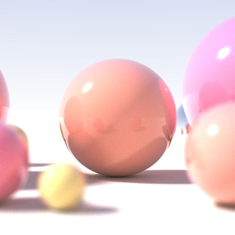
Ray tracing is capable of simulating a variety of optical effects,[3] such as reflection, refraction, soft shadows, scattering, depth of field, motion blur, caustics, ambient occlusion and dispersion phenomena (such as chromatic aberration). It can also be used to trace the path of sound waves in a similar fashion to light waves, making it a viable option for more immersive sound design in video games by rendering realistic reverberation and echoes.[4] In fact, any physical wave or particle phenomenon with approximately linear motion can be simulated with ray tracing.
Ray tracing-based rendering techniques that involve sampling light over a domain generate rays or using denoising techniques.[incomprehensible]
History
[edit]

The idea of ray tracing comes from as early as the 16th century, when it was described by Albrecht Dürer, who is credited for its invention.[5] Dürer described multiple techniques for projecting 3-D scenes onto an image plane. Some of these project chosen geometry onto the image plane, as is done with rasterization today. Others determine what geometry is visible along a given ray, as is done with ray tracing.[6][7]
Using a computer for ray tracing to generate shaded pictures was first accomplished by Arthur Appel in 1968.[8] Appel used ray tracing for primary visibility (determining the closest surface to the camera at each image point) by tracing a ray through each point to be shaded into the scene to identify the visible surface. The closest surface intersected by the ray was the visible one. This non-recursive ray tracing-based rendering algorithm is today called "ray casting". His algorithm then traced secondary rays to the light source from each point being shaded to determine whether the point was in shadow or not.
Later, in 1971, Goldstein and Nagel of MAGI (Mathematical Applications Group, Inc.)[9] published "3-D Visual Simulation", wherein ray tracing was used to make shaded pictures of solids. At the ray-surface intersection point found, they computed the surface normal and, knowing the position of the light source, computed the brightness of the pixel on the screen. Their publication describes a short (30-second) film "made using the University of Maryland's display hardware outfitted with a 16mm camera. The film showed the helicopter and a simple ground-level gun emplacement. The helicopter was programmed to undergo a series of maneuvers including turns, take-offs, and landings, etc., until it eventually is shot down and crashed." A CDC 6600 computer was used. MAGI produced an animation video called MAGI/SynthaVision Sampler in 1974.[10]

Another early instance of ray casting came in 1976, when Scott Roth created a flip book animation in Bob Sproull's computer graphics course at Caltech. The scanned pages are shown as a video in the accompanying image. Roth's computer program noted an edge point at a pixel location if the ray intersected a bounded plane different from that of its neighbors. Of course, a ray could intersect multiple planes in space, but only the surface point closest to the camera was noted as visible. The platform was a DEC PDP-10, a Tektronix storage-tube display, and a printer which would create an image of the display on rolling thermal paper. Roth extended the framework, introduced the term ray casting in the context of computer graphics and solid modeling, and in 1982 published his work while at GM Research Labs.[11]
Turner Whitted was the first to show recursive ray tracing for mirror reflection and for refraction through translucent objects, with an angle determined by the solid's index of refraction, and to use ray tracing for anti-aliasing.[12] Whitted also showed ray traced shadows. He produced a recursive ray-traced film called The Compleat Angler[13] in 1979 while an engineer at Bell Labs. Whitted's deeply recursive ray tracing algorithm reframed rendering from being primarily a matter of surface visibility determination to being a matter of light transport. His paper inspired a series of subsequent work by others that included distribution ray tracing and finally unbiased path tracing, which provides the rendering equation framework that has allowed computer-generated imagery to be faithful to reality.
For decades, global illumination in major films using computer-generated imagery was approximated with additional lights. Ray tracing-based rendering eventually changed that by enabling physically-based light transport. Early feature films rendered entirely using path tracing include Monster House (2006), Cloudy with a Chance of Meatballs (2009),[14] and Monsters University (2013).[15]
Algorithm overview
[edit]

Optical ray tracing describes a method for producing visual images constructed in 3-D computer graphics environments, with more photorealism than either ray casting or scanline rendering techniques. It works by tracing a path from an imaginary eye through each pixel in a virtual screen, and calculating the color of the object visible through it.
Scenes in ray tracing are described mathematically by a programmer or by a visual artist (normally using intermediary tools). Scenes may also incorporate data from images and models captured by means such as digital photography.
Typically, each ray must be tested for intersection with some subset of all the objects in the scene. Once the nearest object has been identified, the algorithm will estimate the incoming light at the point of intersection, examine the material properties of the object, and combine this information to calculate the final color of the pixel. Certain illumination algorithms and reflective or translucent materials may require more rays to be re-cast into the scene.
It may at first seem counterintuitive or "backward" to send rays away from the camera, rather than into it (as actual light does in reality), but doing so is many orders of magnitude more efficient. Since the overwhelming majority of light rays from a given light source do not make it directly into the viewer's eye, a "forward" simulation could potentially waste a tremendous amount of computation on light paths that are never recorded.
Therefore, the shortcut taken in ray tracing is to presuppose that a given ray intersects the view frame. After either a maximum number of reflections or a ray traveling a certain distance without intersection, the ray ceases to travel and the pixel's value is updated.
Calculate rays for rectangular viewport
[edit]On input we have (in calculation we use vector normalization and cross product):
- eye position
- target position
- field of view - for humans, we can assume
- numbers of square pixels on viewport vertical and horizontal direction
- numbers of actual pixel
- vertical vector which indicates where is up and down, usually - roll component which determine viewport rotation around point C (where the axis of rotation is the ET section)


![{\displaystyle \theta \in [0,\pi ]}](https://wikimedia.org/api/rest_v1/media/math/render/svg/c833964ea08aa30df8b6f56664461a5499b38144)




![{\displaystyle {\vec {v}}=[0,1,0]}](https://wikimedia.org/api/rest_v1/media/math/render/svg/8886f18114c9ba99a355b19eb4c8e075524d22b3)

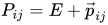
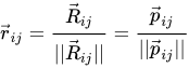
The idea is to find the position of each viewport pixel center which allows us to find the line going from eye through that pixel and finally get the ray described by point and vector (or its normalization ). First we need to find the coordinates of the bottom left viewport pixel and find the next pixel by making a shift along directions parallel to viewport (vectors , ) multiplied by the size of the pixel. Below we introduce formulas which include distance between the eye and the viewport. However, this value will be reduced during ray normalization (so you might as well accept that and remove it from calculations).


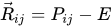


Pre-calculations: let's find and normalize vector and vectors which are parallel to the viewport (all depicted on above picture)




note that viewport center , next we calculate viewport sizes divided by 2 including inverse aspect ratio
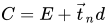



and then we calculate next-pixel shifting vectors along directions parallel to viewport (), and left bottom pixel center



Calculations: note and ray so


Detailed description of ray tracing computer algorithm and its genesis
[edit]What happens in nature (simplified)
[edit]In nature, a light source emits a ray of light which travels, eventually, to a surface that interrupts its progress. One can think of this "ray" as a stream of photons traveling along the same path. In a perfect vacuum this ray will be a straight line (ignoring relativistic effects). Any combination of four things might happen with this light ray: absorption, reflection, refraction and fluorescence. A surface may absorb part of the light ray, resulting in a loss of intensity of the reflected and/or refracted light. It might also reflect all or part of the light ray, in one or more directions. If the surface has any transparent or translucent properties, it refracts a portion of the light beam into itself in a different direction while absorbing some (or all) of the spectrum (and possibly altering the color). Less commonly, a surface may absorb some portion of the light and fluorescently re-emit the light at a longer wavelength color in a random direction, though this is rare enough that it can be discounted from most rendering applications. Between absorption, reflection, refraction and fluorescence, all of the incoming light must be accounted for, and no more. A surface cannot, for instance, reflect 66% of an incoming light ray, and refract 50%, since the two would add up to be 116%. From here, the reflected and/or refracted rays may strike other surfaces, where their absorptive, refractive, reflective and fluorescent properties again affect the progress of the incoming rays. Some of these rays travel in such a way that they hit our eye, causing us to see the scene and so contribute to the final rendered image.
Ray casting algorithm
[edit]The idea behind ray casting, the predecessor to recursive ray tracing, is to trace rays from the eye, one per pixel, and find the closest object blocking the path of that ray. Think of an image as a screen-door, with each square in the screen being a pixel. This is then the object the eye sees through that pixel. Using the material properties and the effect of the lights in the scene, this algorithm can determine the shading of this object. The simplifying assumption is made that if a surface faces a light, the light will reach that surface and not be blocked or in shadow. The shading of the surface is computed using traditional 3-D computer graphics shading models. One important advantage ray casting offered over older scanline algorithms was its ability to easily deal with non-planar surfaces and solids, such as cones and spheres. If a mathematical surface can be intersected by a ray, it can be rendered using ray casting. Elaborate objects can be created by using solid modeling techniques and easily rendered.
Volume ray casting algorithm
[edit]In the method of volume ray casting, each ray is traced so that color and/or density can be sampled along the ray and then be combined into a final pixel color. This is often used when objects cannot be easily represented by explicit surfaces (such as triangles), for example when rendering clouds or 3-D medical scans.

SDF ray marching algorithm
[edit]In SDF ray marching, or sphere tracing,[16] each ray is traced in multiple steps to approximate an intersection point between the ray and a surface defined by a signed distance function (SDF). The SDF is evaluated for each iteration in order to be able take as large steps as possible without missing any part of the surface. A threshold is used to cancel further iteration when a point is reached that is close enough to the surface. This method is often used for 3-D fractal rendering.[17]
Recursive ray tracing algorithm
[edit]


Earlier algorithms traced rays from the eye into the scene until they hit an object, but determined the ray color without recursively tracing more rays. Recursive ray tracing continues the process. When a ray hits a surface, additional rays may be cast because of reflection, refraction, and shadow.:[18]
- A reflection ray is traced in the mirror-reflection direction. The closest object it intersects is what will be seen in the reflection.
- A refraction ray traveling through transparent material works similarly, with the addition that a refractive ray could be entering or exiting a material. Turner Whitted extended the mathematical logic for rays passing through a transparent solid to include the effects of refraction.[19]
- A shadow ray is traced toward each light. If any opaque object is found between the surface and the light, the surface is in shadow and the light does not illuminate it.
These recursive rays add more realism to ray-traced images.
Advantages over other rendering methods
[edit]Ray tracing-based rendering's popularity stems from its basis in a realistic simulation of light transport, as compared to other rendering methods, such as rasterization, which focuses more on the realistic simulation of geometry. Effects such as reflections and shadows, which are difficult to simulate using other algorithms, are a natural result of the ray tracing algorithm. The computational independence of each ray makes ray tracing amenable to a basic level of parallelization,[20] but the divergence of ray paths makes high utilization under parallelism quite difficult to achieve in practice.[21]
Disadvantages
[edit]A serious disadvantage of ray tracing is performance, though it can in theory be faster than traditional scanline rendering, depending on scene complexity vs. number of pixels on-screen. Until the late 2010s, ray tracing in real time was usually considered impossible on consumer hardware for nontrivial tasks. Scanline algorithms and other algorithms use data coherence to share computations between pixels, while ray tracing normally starts the process anew, treating each eye ray separately. However, this separation offers other advantages, such as the ability to shoot more rays as needed to perform spatial anti-aliasing and improve image quality where needed.
Whitted-style recursive ray tracing handles interreflection and optical effects such as refraction, but is not generally photorealistic. Improved realism occurs when the rendering equation is fully evaluated, as the equation conceptually includes every physical effect of light flow. However, this is infeasible given the computing resources required, and the limitations on geometric and material modeling fidelity. Path tracing is an algorithm for evaluating the rendering equation and thus gives a higher-fidelity simulations of real-world lighting.
Reversed direction of traversal of scene by the rays
[edit]The process of shooting rays from the eye to the light source to render an image is sometimes called backwards ray tracing, since it is the opposite direction photons actually travel. However, there is confusion with this terminology. Early ray tracing was always done from the eye, and early researchers such as James Arvo used the term backwards ray tracing to mean shooting rays from the lights and gathering the results. Therefore, it is clearer to distinguish eye-based versus light-based ray tracing.
While the direct illumination is generally best sampled using eye-based ray tracing, certain indirect effects can benefit from rays generated from the lights. Caustics are bright patterns caused by the focusing of light off a wide reflective region onto a narrow area of (near-)diffuse surface. An algorithm that casts rays directly from lights onto reflective objects, tracing their paths to the eye, will better sample this phenomenon. This integration of eye-based and light-based rays is often expressed as bidirectional path tracing, in which paths are traced from both the eye and lights, and the paths subsequently joined by a connecting ray after some length.[22][23]
Photon mapping is another method that uses both light-based and eye-based ray tracing; in an initial pass, energetic photons are traced along rays from the light source so as to compute an estimate of radiant flux as a function of 3-dimensional space (the eponymous photon map itself). In a subsequent pass, rays are traced from the eye into the scene to determine the visible surfaces, and the photon map is used to estimate the illumination at the visible surface points.[24][25] The advantage of photon mapping versus bidirectional path tracing is the ability to achieve significant reuse of photons, reducing computation, at the cost of statistical bias.
An additional problem occurs when light must pass through a very narrow aperture to illuminate the scene (consider a darkened room, with a door slightly ajar leading to a brightly lit room), or a scene in which most points do not have direct line-of-sight to any light source (such as with ceiling-directed light fixtures or torchieres). In such cases, only a very small subset of paths will transport energy; Metropolis light transport is a method which begins with a random search of the path space, and when energetic paths are found, reuses this information by exploring the nearby space of rays.[26]

To the right is an image showing a simple example of a path of rays recursively generated from the camera (or eye) to the light source using the above algorithm. A diffuse surface reflects light in all directions.
First, a ray is created at an eyepoint and traced through a pixel and into the scene, where it hits a diffuse surface. From that surface, the algorithm recursively generates a reflection ray, which is traced through the scene, where it hits another diffuse surface. Finally, another reflection ray is generated and traced through the scene, where it hits the light source and is absorbed. The color of the pixel now depends on the colors of the first and second diffuse surfaces and the color of the light emitted from the light source. For example, if the light source emitted white light and the two diffuse surfaces were blue, then the resulting color of the pixel is blue.
Example
[edit].png)
As a demonstration of the principles involved in ray tracing, consider how one would find the intersection between a ray and a sphere. This is merely the math behind the line–sphere intersection and the subsequent determination of the color of the pixel being calculated. There is, of course, far more to the general process of ray tracing, but this demonstrates an example of the algorithms used.
In vector notation, the equation of a sphere with center and radius is


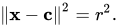
Any point on a ray starting from point with direction (here is a unit vector) can be written as


where is its distance between and . In our problem, we know , , (e.g. the position of a light source) and , and we need to find . Therefore, we substitute for :



Let for simplicity; then

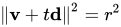


Knowing that d is a unit vector allows us this minor simplification:

This quadratic equation has solutions

The two values of found by solving this equation are the two ones such that are the points where the ray intersects the sphere.

Any value which is negative does not lie on the ray, but rather in the opposite half-line (i.e. the one starting from with opposite direction).
If the quantity under the square root (the discriminant) is negative, then the ray does not intersect the sphere.
Let us suppose now that there is at least a positive solution, and let be the minimal one. In addition, let us suppose that the sphere is the nearest object on our scene intersecting our ray, and that it is made of a reflective material. We need to find in which direction the light ray is reflected. The laws of reflection state that the angle of reflection is equal and opposite to the angle of incidence between the incident ray and the normal to the sphere.
The normal to the sphere is simply
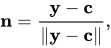
where is the intersection point found before. The reflection direction can be found by a reflection of with respect to , that is



Thus the reflected ray has equation

Now we only need to compute the intersection of the latter ray with our field of view, to get the pixel which our reflected light ray will hit. Lastly, this pixel is set to an appropriate color, taking into account how the color of the original light source and that of the sphere are combined by the reflection.
Adaptive depth control
[edit]Adaptive depth control means that the renderer stops generating reflected/transmitted rays when the computed intensity becomes less than a certain threshold. There must always be a set maximum depth or else the program would generate an infinite number of rays. But it is not always necessary to go to the maximum depth if the surfaces are not highly reflective. To test for this the ray tracer must compute and keep the product of the global and reflection coefficients as the rays are traced.
Example: let Kr = 0.5 for a set of surfaces. Then from the first surface the maximum contribution is 0.5, for the reflection from the second: 0.5 × 0.5 = 0.25, the third: 0.25 × 0.5 = 0.125, the fourth: 0.125 × 0.5 = 0.0625, the fifth: 0.0625 × 0.5 = 0.03125, etc. In addition we might implement a distance attenuation factor such as 1/D2, which would also decrease the intensity contribution.
For a transmitted ray we could do something similar but in that case the distance traveled through the object would cause even faster intensity decrease. As an example of this, Hall & Greenberg found that even for a very reflective scene, using this with a maximum depth of 15 resulted in an average ray tree depth of 1.7.[27]
Bounding volumes
[edit]Enclosing groups of objects in sets of bounding volume hierarchies (BVH) decreases the amount of computations required for ray tracing. A cast ray is first tested for an intersection with the bounding volume, and then if there is an intersection, the volume is recursively divided until the ray hits the object. The best type of bounding volume will be determined by the shape of the underlying object or objects. For example, if the objects are long and thin, then a sphere will enclose mainly empty space compared to a box. Boxes are also easier to generate hierarchical bounding volumes.
Note that using a hierarchical system like this (assuming it is done carefully) changes the intersection computational time from a linear dependence on the number of objects to something between linear and a logarithmic dependence. This is because, for a perfect case, each intersection test would divide the possibilities by two, and result in a binary tree type structure. Spatial subdivision methods, discussed below, try to achieve this. Furthermore, this acceleration structure makes the ray-tracing computation output-sensitive. I.e. the complexity of the ray intersection calculations depends on the number of objects that actually intersect the rays and not (only) on the number of objects in the scene.
Kay & Kajiya give a list of desired properties for hierarchical bounding volumes:
- Subtrees should contain objects that are near each other and the further down the tree the closer should be the objects.
- The volume of each node should be minimal.
- The sum of the volumes of all bounding volumes should be minimal.
- Greater attention should be placed on the nodes near the root since pruning a branch near the root will remove more potential objects than one farther down the tree.
- The time spent constructing the hierarchy should be much less than the time saved by using it.
Interactive ray tracing
[edit]The first implementation of an interactive ray tracer was the LINKS-1 Computer Graphics System built in 1982 at Osaka University's School of Engineering, by professors Ohmura Kouichi, Shirakawa Isao and Kawata Toru with 50 students.[citation needed] It was a massively parallel processing computer system with 514 microprocessors (257 Zilog Z8001s and 257 iAPX 86s), used for 3-D computer graphics with high-speed ray tracing. According to the Information Processing Society of Japan: "The core of 3-D image rendering is calculating the luminance of each pixel making up a rendered surface from the given viewpoint, light source, and object position. The LINKS-1 system was developed to realize an image rendering methodology in which each pixel could be parallel processed independently using ray tracing. By developing a new software methodology specifically for high-speed image rendering, LINKS-1 was able to rapidly render highly realistic images." It was used to create an early 3-D planetarium-like video of the heavens made completely with computer graphics. The video was presented at the Fujitsu pavilion at the 1985 International Exposition in Tsukuba."[28] It was the second system to do so after the Evans & Sutherland Digistar in 1982. The LINKS-1 was claimed by the designers to be the world's most powerful computer in 1984.[29]
The next interactive ray tracer, and the first known to have been labeled "real-time" was credited at the 2005 SIGGRAPH computer graphics conference as being the REMRT/RT tools developed in 1986 by Mike Muuss for the BRL-CAD solid modeling system. Initially published in 1987 at USENIX, the BRL-CAD ray tracer was an early implementation of a parallel network distributed ray tracing system that achieved several frames per second in rendering performance.[30] This performance was attained by means of the highly optimized yet platform independent LIBRT ray tracing engine in BRL-CAD and by using solid implicit CSG geometry on several shared memory parallel machines over a commodity network. BRL-CAD's ray tracer, including the REMRT/RT tools, continue to be available and developed today as open source software.[31]
Since then, there have been considerable efforts and research towards implementing ray tracing at real-time speeds for a variety of purposes on stand-alone desktop configurations. These purposes include interactive 3-D graphics applications such as demoscene productions, computer and video games, and image rendering. Some real-time software 3-D engines based on ray tracing have been developed by hobbyist demo programmers since the late 1990s.[32]
In 1999 a team from the University of Utah, led by Steven Parker, demonstrated interactive ray tracing live at the 1999 Symposium on Interactive 3D Graphics. They rendered a 35 million sphere model at 512 by 512 pixel resolution, running at approximately 15 frames per second on 60 CPUs.[33]
The Open RT project included a highly optimized software core for ray tracing along with an OpenGL-like API in order to offer an alternative to the current rasterization based approach for interactive 3-D graphics. Ray tracing hardware, such as the experimental Ray Processing Unit developed by Sven Woop at the Saarland University, was designed to accelerate some of the computationally intensive operations of ray tracing.
The idea that video games could ray trace their graphics in real time received media attention in the late 2000s. During that time, a researcher named Daniel Pohl, under the guidance of graphics professor Philipp Slusallek and in cooperation with the Erlangen University and Saarland University in Germany, equipped Quake III and Quake IV with an engine he programmed himself, which Saarland University then demonstrated at CeBIT 2007.[34] Intel, a patron of Saarland, became impressed enough that it hired Pohl and embarked on a research program dedicated to ray traced graphics, which it saw as justifying increasing the number of its processors' cores.[35]: 99–100 [36] On June 12, 2008, Intel demonstrated a special version of Enemy Territory: Quake Wars, titled Quake Wars: Ray Traced, using ray tracing for rendering, running in basic HD (720p) resolution. ETQW operated at 14–29 frames per second on a 16-core (4 socket, 4 core) Xeon Tigerton system running at 2.93 GHz.[37]
At SIGGRAPH 2009, Nvidia announced OptiX, a free API for real-time ray tracing on Nvidia GPUs. The API exposes seven programmable entry points within the ray tracing pipeline, allowing for custom cameras, ray-primitive intersections, shaders, shadowing, etc. This flexibility enables bidirectional path tracing, Metropolis light transport, and many other rendering algorithms that cannot be implemented with tail recursion.[38] OptiX-based renderers are used in Autodesk Arnold, Adobe AfterEffects, Bunkspeed Shot, Autodesk Maya, 3ds max, and many other renderers.
In 2014, a demo of the PlayStation 4 game The Tomorrow Children, developed by Q-Games and Japan Studio, demonstrated new lighting techniques developed by Q-Games, notably cascaded voxel cone ray tracing, which simulates lighting in real-time and uses more realistic reflections rather than screen space reflections.[39]
Nvidia introduced their GeForce RTX and Quadro RTX GPUs in September 2018, based on the Turing architecture that allows for hardware-accelerated ray tracing. The Nvidia hardware uses a separate functional block, publicly called an "RT core". This unit is somewhat comparable to a texture unit in size, latency, and interface to the processor core. The unit features BVH traversal, compressed BVH node decompression, ray-AABB intersection testing, and ray-triangle intersection testing.[40] The GeForce RTX, in the form of models 2080 and 2080 Ti, became the first consumer-oriented brand of graphics card that can perform ray tracing in real time,[41] and, in November 2018, Electronic Arts' Battlefield V became the first game to take advantage of its ray tracing capabilities, which it achieves via Microsoft's new API, DirectX Raytracing.[42] AMD, which already offered interactive ray tracing on top of OpenCL through its Radeon ProRender,[43][44] unveiled in October 2020 the Radeon RX 6000 series, its second generation Navi GPUs with support for hardware-accelerated ray tracing at an online event.[45][46][47][48][49] Subsequent games that render their graphics by such means appeared since, which has been credited to the improvements in hardware and efforts to make more APIs and game engines compatible with the technology.[50] Current home gaming consoles implement dedicated ray tracing hardware components in their GPUs for real-time ray tracing effects, which began with the ninth-generation consoles PlayStation 5, Xbox Series X and Series S.[51][52][53][54][55]
On 4 November, 2021, Imagination Technologies announced their IMG CXT GPU with hardware-accelerated ray tracing.[56][57] On January 18, 2022, Samsung announced their Exynos 2200 AP SoC with hardware-accelerated ray tracing.[58] On June 28, 2022, Arm announced their Immortalis-G715 with hardware-accelerated ray tracing.[59] On November 16, 2022, Qualcomm announced their Snapdragon 8 Gen 2 with hardware-accelerated ray tracing.[60][61]
On September 12, 2023 Apple introduced hardware-accelerated ray tracing in its chip designs, beginning with the A17 Pro chip for iPhone 15 Pro models.[62][63] Later the same year, Apple released M3 family of processors with HW enabled ray tracing support.[64] Currently, this technology is accessible across iPhones, iPads, and Mac computers via the Metal API. Apple reports up to a 4x performance increase over previous software-based ray tracing on the phone[63] and up to 2.5x faster comparing M3 to M1 chips.[64] The hardware implementation includes acceleration structure traversal and dedicated ray-box intersections, and the API supports RayQuery (Inline Ray Tracing) as well as RayPipeline features.[65]
Computational complexity
[edit]Various complexity results have been proven for certain formulations of the ray tracing problem. In particular, if the decision version of the ray tracing problem is defined as follows[66] – given a light ray's initial position and direction and some fixed point, does the ray eventually reach that point, then the referenced paper proves the following results:
- Ray tracing in 3-D optical systems with a finite set of reflective or refractive objects represented by a system of rational quadratic inequalities is undecidable.
- Ray tracing in 3-D optical systems with a finite set of refractive objects represented by a system of rational linear inequalities is undecidable.
- Ray tracing in 3-D optical systems with a finite set of rectangular reflective or refractive objects is undecidable.
- Ray tracing in 3-D optical systems with a finite set of reflective or partially reflective objects represented by a system of linear inequalities, some of which can be irrational is undecidable.
- Ray tracing in 3-D optical systems with a finite set of reflective or partially reflective objects represented by a system of rational linear inequalities is PSPACE-hard.
- For any dimension equal to or greater than 2, ray tracing with a finite set of parallel and perpendicular reflective surfaces represented by rational linear inequalities is in PSPACE.
Software architecture
[edit]See also
[edit]References
[edit]- ^ Shirley, Peter (July 9, 2003). Realistic Ray Tracing. A K Peters/CRC Press; 2nd edition. ISBN 978-1568814612.
- ^ "Sponsored Feature: Changing the Game - Experimental Cloud-Based Ray Tracing". www.gamasutra.com. Archived from the original on May 9, 2012. Retrieved March 18, 2021.
- ^ "Disney explains why its 2D animation looks so realistic". Engadget. Retrieved March 18, 2021.[dead link]
- ^ Kastbauer, Damian (January 28, 2010). "The Next Big Steps In Game Sound Design". Gamasutra. Archived from the original on May 9, 2012. Retrieved March 18, 2021.
- ^ Georg Rainer Hofmann (1990). "Who invented ray tracing?". The Visual Computer. 6 (3): 120–124. doi:10.1007/BF01911003. S2CID 26348610..
- ^ Steve Luecking (2013). "Dürer, drawing, and digital thinking - 2013 FATE Conference". brian-curtis.com. Retrieved August 13, 2020.
- ^ Steve Luecking. "Stephen J Luecking". Retrieved August 13, 2020.
- ^ Appel, Arthur (April 30, 1968). "Some techniques for shading machine renderings of solids". Proceedings of the April 30--May 2, 1968, spring joint computer conference on - AFIPS '68 (Spring) (PDF). pp. 37–45. doi:10.1145/1468075.1468082. S2CID 207171023.
- ^ Goldstein, Robert; Nagel, Roger (January 1971), "3-D Visual simulation", Simulation, 16 (1): 25–31, doi:10.1177/003754977101600104, S2CID 122824395
- ^ Syntha Vision Sampler. 1974 – via Internet Archive.
- ^ Roth, Scott D. (February 1982), "Ray Casting for Modeling Solids", Computer Graphics and Image Processing, 18 (2): 109–144, doi:10.1016/0146-664X(82)90169-1
- ^ Whitted T. (1979) An Improved Illumination Model for Shaded Display. Proceedings of the 6th annual conference on Computer graphics and interactive techniques
- ^ The Compleat Angler. Bell Laboratories. 1978 – via Internet Archive.
- ^ "Food for Laughs". Computer Graphics World.
- ^ M.s (May 28, 2013). "This Animated Life: Pixar's Lightspeed Brings New Light to Monsters University". This Animated Life. Retrieved May 26, 2020.
- ^ Hart, John C. (June 1995), "Sphere Tracing: A Geometric Method for the Antialiased Ray Tracing of Implicit Surfaces" (PDF), The Visual Computer
- ^ Hart, John C.; Sandin, Daniel J.; Kauffman, Louis H. (July 1989), "Ray Tracing Deterministic 3-D Fractals" (PDF), Computer Graphics, 23 (3): 289–296, doi:10.1145/74334.74363
- ^ Tomas Nikodym (June 2010). "Ray Tracing Algorithm For Interactive Applications" (PDF). Czech Technical University, FEE. Archived from the original (PDF) on March 3, 2016.
- ^ Whitted, T. (1979). "An Improved Illumination Model for Shaded Display". Proceedings of the 6th annual conference on Computer graphics and interactive techniques. Association for Computing Machinery. CiteSeerX 10.1.1.156.1534. ISBN 0-89791-004-4.
- ^ Chalmers, A.; Davis, T.; Reinhard, E. (2002). Practical Parallel Rendering. AK Peters. ISBN 1-56881-179-9.
- ^ Aila, Timo; Laine, Samulii (2009). "Understanding the Efficiency of Ray Traversal on GPUs". HPG '09: Proceedings of the Conference on High Performance Graphics 2009. pp. 145–149. doi:10.1145/1572769.1572792. ISBN 9781605586038. S2CID 15392840.
- ^ Eric P. Lafortune and Yves D. Willems (December 1993). "Bi-Directional Path Tracing". Proceedings of Compugraphics '93: 145–153.
- ^ Péter Dornbach (1998). "Implementation of bidirectional ray tracing algorithm" (PDF). Retrieved June 11, 2008.
- ^ Global Illumination using Photon Maps Archived 2008-08-08 at the Wayback Machine
- ^ "Photon Mapping - Zack Waters".
- ^ Veach, Eric; Guibas, Leonidas J. (1997). "Metropolis Light Transport". SIGGRAPH '97: Proceedings of the 24th annual conference on Computer graphics and interactive techniques. pp. 65–76. doi:10.1145/258734.258775. ISBN 0897918967. S2CID 1832504.
- ^ Hall, Roy A.; Greenberg, Donald P. (November 1983). "A Testbed for Realistic Image Synthesis". IEEE Computer Graphics and Applications. 3 (8): 10–20. CiteSeerX 10.1.1.131.1958. doi:10.1109/MCG.1983.263292. S2CID 9594422.
- ^ "【Osaka University 】 LINKS-1 Computer Graphics System". IPSJ Computer Museum. Information Processing Society of Japan. Retrieved November 15, 2018.
- ^ Defanti, Thomas A. (1984). Advances in computers. Volume 23 (PDF). Academic Press. p. 121. ISBN 0-12-012123-9.
- ^ See Proceedings of 4th Computer Graphics Workshop, Cambridge, MA, USA, October 1987. Usenix Association, 1987. pp 86–98.
- ^ "About BRL-CAD". Archived from the original on September 1, 2009. Retrieved January 18, 2019.
- ^ Piero Foscari. "The Realtime Raytracing Realm". ACM Transactions on Graphics. Retrieved September 17, 2007.
- ^ Parker, Steven; Martin, William (April 26, 1999). "Interactive ray tracing". Proceedings of the 1999 symposium on Interactive 3-D graphics. I3D '99. Vol. 5. pp. 119–126. CiteSeerX 10.1.1.6.8426. doi:10.1145/300523.300537. ISBN 1581130821. S2CID 4522715. Retrieved October 30, 2019.
- ^ Mark Ward (March 16, 2007). "Rays light up life-like graphics". BBC News. Retrieved September 17, 2007.
- ^ Peddie, Jon (2019). Ray Tracing: A Tool for All. Springer Nature Switzerland. ISBN 978-3-030-17490-3. Retrieved November 2, 2022.
- ^ Abi-Chahla, Fedy (July 22, 2009). "When Will Ray Tracing Replace Rasterization?". Tom's Hardware. Archived from the original on November 3, 2022. Retrieved November 4, 2022.
- ^ Valich, Theo (June 12, 2008). "Intel converts ET: Quake Wars to ray tracing". TG Daily. Archived from the original on October 2, 2008. Retrieved June 16, 2008.
- ^ Nvidia (October 18, 2009). "Nvidia OptiX". Nvidia. Retrieved November 6, 2009.
- ^ Cuthbert, Dylan (October 24, 2015). "Creating the beautiful, ground-breaking visuals of The Tomorrow Children on PS4". PlayStation Blog. Retrieved December 7, 2015.
- ^ Kilgariff, Emmett; Moreton, Henry; Stam, Nick; Bell, Brandon (September 14, 2018). "NVIDIA Turing Architecture In-Depth". Nvidia Developer. Archived from the original on November 13, 2022. Retrieved November 13, 2022.
- ^ Takahashi, Dean (August 20, 2018). "Nvidia unveils GeForce RTX graphics chips for real-time ray tracing games". VentureBeat. Archived from the original on November 13, 2022. Retrieved November 13, 2022.
- ^ Chacos, Brad (November 14, 2018). "RTX on! Battlefield V becomes the first game to support DXR real-time ray tracing". PCWorld. Archived from the original on November 13, 2022. Retrieved November 13, 2018.
- ^ "Real-Time Ray Tracing with Radeon ProRender". GPUOpen. March 20, 2018. Archived from the original on November 13, 2022. Retrieved November 13, 2022.
- ^ Harada, Takahiro (November 23, 2020). "Hardware-Accelerated Ray Tracing in AMD Radeon™ ProRender 2.0". GPUOpen. Archived from the original on November 13, 2022. Retrieved November 13, 2022.
- ^ Garreffa, Anthony (September 9, 2020). "AMD to reveal next-gen Big Navi RDNA 2 graphics cards on October 28". TweakTown. Retrieved September 9, 2020.
- ^ Lyles, Taylor (September 9, 2020). "AMD's next-generation Zen 3 CPUs and Radeon RX 6000 'Big Navi' GPU will be revealed next month". The Verge. Retrieved September 10, 2020.
- ^ "AMD Teases Radeon RX 6000 Card Performance Numbers: Aiming For 3080?". anandtech.com. AnandTech. October 8, 2020. Archived from the original on October 8, 2020. Retrieved October 25, 2020.
- ^ "AMD Announces Ryzen "Zen 3" and Radeon "RDNA2" Presentations for October: A New Journey Begins". anandtech.com. AnandTech. September 9, 2020. Archived from the original on September 10, 2020. Retrieved October 25, 2020.
- ^ Judd, Will (October 28, 2020). "AMD unveils three Radeon 6000 graphics cards with ray tracing and RTX-beating performance". Eurogamer. Retrieved October 28, 2020.
- ^ Marrs, Adam; Shirley, Peter; Wald, Ingo (2021). Ray Tracing Gems II: Next Generation Real-Time Rendering with DXR, Vulkan, and OptiX. Apress. pp. 213–214, 791–792. hdl:20.500.12657/50334. ISBN 9781484271858.
- ^ Warren, Tom (June 8, 2019). "Microsoft hints at next-generation Xbox 'Scarlet' in E3 teasers". The Verge. Retrieved October 8, 2019.
- ^ Chaim, Gartenberg (October 8, 2019). "Sony confirms PlayStation 5 name, holiday 2020 release date". The Verge. Retrieved October 8, 2019.
- ^ Warren, Tom (February 24, 2020). "Microsoft reveals more Xbox Series X specs, confirms 12 teraflops GPU". The Verge. Retrieved February 25, 2020.
- ^ Warren, Tom (September 9, 2020). "Microsoft reveals Xbox Series S specs, promises four times the processing power of Xbox One". The Verge. Retrieved September 9, 2020.
- ^ Vandervell, Andy (January 4, 2020). "Making sense of the rampant Xbox Series X rumour mill". Wired. Archived from the original on November 13, 2022. Retrieved November 13, 2022.
- ^ 93digital (November 4, 2021). "Imagination launches the most advanced ray tracing GPU". Imagination. Retrieved September 17, 2023.
{{cite web}}: CS1 maint: numeric names: authors list (link) - ^ "Ray Tracing". Imagination. Retrieved September 17, 2023.
- ^ "Samsung Introduces Game Changing Exynos 2200 Processor With Xclipse GPU Powered by AMD RDNA 2 Architecture". news.samsung.com. Retrieved September 17, 2023.
- ^ "Gaming Performance Unleashed with Arm's new GPUs - Announcements - Arm Community blogs - Arm Community". community.arm.com. June 28, 2022. Retrieved September 17, 2023.
- ^ "Snapdragon 8 Gen 2 Defines a New Standard for Premium Smartphones". www.qualcomm.com. Retrieved September 17, 2023.
- ^ "New, Snapdragon 8 Gen 2: 8 extraordinary mobile experiences, unveiled". www.qualcomm.com. Retrieved September 17, 2023.
- ^ Bonshor, Ryan Smith, Gavin. "The Apple 2023 Fall iPhone Event Live Blog (Starts at 10am PT/17:00 UTC)". www.anandtech.com. Archived from the original on September 12, 2023. Retrieved September 17, 2023.
{{cite web}}: CS1 maint: multiple names: authors list (link) - ^ a b "Apple unveils iPhone 15 Pro and iPhone 15 Pro Max". Apple Newsroom. Retrieved October 27, 2024.
- ^ a b "Apple unveils M3, M3 Pro, and M3 Max, the most advanced chips for a personal computer". Apple Newsroom. Retrieved October 27, 2024.
- ^ "Discover ray tracing with Metal - WWDC20 - Videos". Apple Developer. Retrieved October 27, 2024.
- ^ "Computability and Complexity of Ray Tracing" (PDF). CS.Duke.edu.
External links
[edit]- Interactive Ray Tracing: The replacement of rasterization?
- The Compleat Angler (1978)
- Writing a Simple Ray Tracer (scratchapixel) Archived February 28, 2015, at the Wayback Machine
- Ray tracing a torus Archived February 12, 2019, at the Wayback Machine
- Ray Tracing in One Weekend Book Series
- Ray Tracing with Voxels - Part 1
Ray tracing (graphics)
View on GrokipediaOverview
Core Principles
Ray tracing is a rendering technique in computer graphics that simulates the physical behavior of light by tracing the paths of rays from the virtual camera through each pixel of the image plane into the scene, computing the color of each pixel based on intersections with scene geometry and subsequent light interactions at those points.[12] This approach allows for realistic rendering of effects such as shadows, reflections, and refractions by modeling how light rays propagate and interact with surfaces.[3] In physical light transport, rays originate from light sources and scatter in all directions, but ray tracing reverses this process for computational efficiency, tracing rays backward from the viewer (or camera) toward the light sources to determine visible contributions.[13] This backward tracing mimics the selective sampling of light paths that reach the observer, reducing the need to simulate all possible light rays in the scene.[14] A ray in ray tracing is mathematically represented in parametric form as , where is the ray's origin point, is its direction vector (typically normalized to unit length), and is a scalar parameter that locates points along the ray.[13] Intersection points occur where satisfies the geometry's implicit equation. For primary rays, which initiate the tracing process, they are generated using a pinhole camera model where the camera is positioned at (the eye point), and the image plane (viewport) is a rectangular grid at a fixed distance from the camera, spanning horizontal and vertical field-of-view angles or dimensions.[15] For a pixel at normalized coordinates in the viewport (where ), the ray direction is computed as in camera space, where is the vertical field of view and aspect is the viewport's aspect ratio; this vector is then normalized to unit length, then transformed to world space if needed.[16] To determine if a ray intersects scene geometry, intersection tests are performed against primitive shapes like spheres or planes, solving for valid values. For a sphere centered at with radius , the intersection solves the quadratic equation derived from substituting the ray equation into the sphere's implicit form , yielding .[17] The discriminant (with , , ) determines real intersections if , and the smallest positive root gives the nearest hit point. Example pseudocode for this test is as follows:function intersectSphere(ray, sphere):
oc = ray.origin - sphere.center
a = dot(ray.direction, ray.direction)
b = 2.0 * dot(oc, ray.direction)
c = dot(oc, oc) - sphere.radius * sphere.radius
discriminant = b * b - 4 * a * c
if discriminant < 0:
return no intersection
t1 = (-b - sqrt(discriminant)) / (2 * a)
t2 = (-b + sqrt(discriminant)) / (2 * a)
if t1 > 0:
return t1 // nearest positive intersection
elif t2 > 0:
return t2
else:
return no intersection
Ray-Scene Interactions
Upon detecting an intersection between a primary ray and a scene object, the ray tracing algorithm computes the precise hit point, the surface normal vector at that location, and the material properties associated with the object.[12] These computations enable subsequent shading and secondary ray generation. To determine the color at the intersection point, a local illumination model evaluates contributions from direct lighting sources. The Phong shading model, an empirical approach, approximates surface appearance through ambient, diffuse, and specular components:History
Origins and Early Concepts
The concept of ray tracing in computer graphics draws its foundational inspiration from geometrical optics in physics, where light is modeled as rays that propagate in straight lines, reflect, and refract upon interacting with surfaces.[21] This simplification of natural light behavior allowed early researchers to simulate realistic visual effects computationally, adapting physical principles to address rendering challenges in digital scenes.[22] One of the earliest applications in computer graphics appeared in Arthur Appel's 1968 work, which introduced ray tracing as a method for hidden surface removal and basic shading in three-dimensional solid models.[2] Appel's algorithm cast rays from the viewpoint through each pixel to determine visible surfaces and compute simple illumination, marking a shift toward more realistic representations beyond mere outlines.[23] This approach efficiently handled complex geometries by tracing rays to identify occlusions and apply tonal shading based on surface normals and light direction.[2] During the 1970s, computer graphics research transitioned from wireframe models—limited to line drawings without depth cues—to shaded renderings that incorporated surface properties and lighting for enhanced realism.[24] This evolution was driven by the need to simulate perceptual depth and material interactions, setting the stage for advanced techniques. A pivotal advancement came in Turner Whitted's 1980 paper, which formalized recursive ray tracing to model reflections and refractions by spawning secondary rays from intersection points, creating a tree-like structure of light paths.[12] Whitted's model extended earlier local illumination methods, enabling the rendering of glossy and transparent effects on both polygonal and curved surfaces.[3] Early ray tracing efforts immediately highlighted significant computational challenges, particularly the high cost of ray-object intersection calculations, which could consume 75-95% of processing time for even modest scenes.[3] Rendering a single image on hardware like the VAX-11/780 often required 44-122 minutes, underscoring the technique's potential for photorealism but limiting its practicality to offline computation.[12] These origins laid the theoretical groundwork for ray tracing, emphasizing its roots in optical simulation while navigating the trade-offs between visual fidelity and efficiency.[3]Evolution and Key Milestones
In the 1990s and early 2000s, ray tracing transitioned from theoretical research to practical integration in film rendering, bolstered by advancements in acceleration structures like kd-trees, which were first adapted for ray tracing in 1985 and refined through subsequent studies on efficient spatial partitioning for complex scenes.[25] Pixar's RenderMan renderer, initially scanline-based, incorporated ray tracing in the mid-2000s, enabling its use in production for the 2006 film Cars, where it handled indirect lighting and reflections across millions of geometric primitives.[26] The 2010s marked a resurgence in ray tracing, propelled by hardware innovations that made real-time applications feasible. NVIDIA introduced the GeForce RTX series in 2018, featuring dedicated RT cores to accelerate ray-triangle intersections and enable real-time ray tracing in games and simulations.[27] AMD countered with its RDNA 2 architecture in 2020, integrating ray accelerators into GPUs for comparable hardware support in DirectX Raytracing (DXR) and Vulkan environments.[28] Path tracing, which extends ray tracing to unbiased global illumination via Monte Carlo sampling, gained traction in film pipelines during this period. Walt Disney Animation Studios debuted its in-house Hyperion renderer—a path-tracing system—for Big Hero 6 in 2014, achieving physically accurate lighting for urban environments with billions of light paths simulated per frame.[29] Entering the 2020s, ray tracing achieved widespread adoption in interactive media, particularly video games. Cyberpunk 2077, released in 2020, showcased ray-traced reflections, shadows, and ambient occlusion, pushing hardware limits and highlighting the technology's role in photorealistic urban scenes.[30] To address performance bottlenecks in real-time contexts, AI-driven denoising emerged as a key enabler; NVIDIA's DLSS 3, launched in 2022, used neural networks to upscale and denoise ray-traced frames, boosting frame rates by up to 4x in supported titles while preserving detail.[31] By 2025, hybrid rasterization-ray tracing pipelines have solidified as the norm in consumer hardware, with consoles like the PlayStation 5 and Xbox Series X—debuted in 2020—employing AMD's RDNA 2-derived GPUs for dynamic ray-traced effects in AAA titles, balancing computational cost with visual realism.[32] NVIDIA's Blackwell architecture, released in January 2025 with the GeForce RTX 50 series, introduced 4th-generation RT cores for up to 2x improved ray tracing performance, while AMD's RDNA 4 architecture, launched in March 2025 with the Radeon RX 9000 series, enhanced ray accelerators for broader adoption.[33][34] Open standards have also evolved significantly; the Vulkan Ray Tracing Extensions, provisionally released in 2020 and finalized in November 2020, now support mature, cross-vendor implementations, facilitating portable ray tracing in diverse ecosystems from mobile to high-end PCs.[35]Fundamental Algorithms
Ray Casting
Ray casting is a foundational rendering technique in computer graphics that simulates visibility by projecting rays from the viewpoint through each pixel of an image plane into the scene to detect the nearest surface intersection. This method determines what objects are visible to the viewer and applies basic local shading to compute pixel colors, serving as a precursor to more advanced ray tracing algorithms. Unlike forward tracing, which originates rays from light sources and is computationally inefficient due to the vast number of photons emitted, ray casting employs backward tracing by launching primary rays solely from the eye position, focusing only on rays that could reach the viewer.[36][37] The algorithm proceeds in a straightforward loop: for each pixel in the image, a ray is generated from the camera's eye point through the pixel's center on the virtual image plane; this ray is then tested for intersections with all objects in the scene, and the closest intersection point is selected to resolve depth and visibility, akin to hidden surface removal in depth buffering. If an intersection occurs, the pixel color is calculated using a local illumination model, such as the Phong shading equation, based on the surface normal, material properties, and direct lighting at that point—without considering indirect effects like shadows unless explicitly added via secondary rays. No recursion is involved, limiting the process to primary eye rays only.[38][39] The following pseudocode illustrates the core ray casting loop for a simple scene:select center of projection (eye) and window on view plane;
for (each pixel in image) {
determine ray direction from eye through pixel [center](/page/Center);
initialize closest distance to [infinity](/page/Infinity);
for (each object in scene) {
compute [intersection](/page/Intersection) with ray;
if ([intersection](/page/Intersection) exists and distance < closest distance) {
update closest distance and record hit point, normal, and object;
}
}
if (hit found) {
compute local shading at hit point using direct lights;
set pixel color to shaded color;
} else {
set pixel color to background color;
}
}
Recursive Ray Tracing
Recursive ray tracing, introduced by Turner Whitted in 1980, extends basic ray casting by recursively generating secondary rays to simulate global illumination effects such as reflections and refractions.[3] In this algorithm, a primary ray from the eye through each pixel intersects the scene, and at the hit point, the shading computation spawns additional rays for specular reflection, transmission (refraction), and shadows toward light sources.[12] This process builds a ray tree where each node represents an intersection, and branches correspond to secondary rays, enabling the rendering of mirrored surfaces and transparent materials that basic ray casting cannot handle.[4] The core of the algorithm lies in the recursive shading function, which combines local illumination with contributions from recursive ray traces. The intensity at an intersection point is computed aswhere is ambient light, the sum accounts for diffuse contributions from light sources with normal and light direction , is the specular reflection term with obtained by recursively tracing a reflected ray, and is the transmission term with from a refracted ray; coefficients , , and control material properties.[3] Shadow rays are cast from the intersection to each light source to check visibility; if any object blocks the ray, the light's contribution is zeroed, preventing self-shadowing.[12] The reflected ray direction follows , and the refracted ray obeys Snell's law, ensuring physically plausible bending at interfaces.[3] To prevent infinite recursion in scenes with highly reflective or refractive materials, termination conditions are enforced. Common limits include a maximum recursion depth of 5-10 bounces, beyond which rays are terminated with a default background color.[42] Additional conditions involve rays that miss all objects (yielding background illumination), total internal reflection during refraction (where the incident angle exceeds the critical angle, spawning a reflection ray instead), or rays at grazing angles where the cosine of the angle between the ray and surface normal falls below a small threshold, avoiding numerical instability and excessive computation.[43] These controls balance realism with computational feasibility, as the number of rays grows exponentially with depth—for instance, each recursive call can spawn up to three secondary rays (reflection, refraction, and multiple shadows).[4] A illustrative example is ray tracing a mirrored sphere illuminated by point lights. The primary ray hits the sphere, spawning a reflection ray that bounces off the surface toward the background or other objects, potentially intersecting a second surface and recursing further; shadow rays from the hit point to each light confirm direct visibility, while the recursion depth limits traces to avoid endless mirroring. This ray tree structure—starting with one primary ray branching into reflection, possible refraction (if transparent), and shadow rays—captures the sphere's reflective highlights and cast shadows accurately.[3] In mimicking natural phenomena, recursive ray tracing excels at approximating specular highlights on glossy surfaces and simple caustics from refractive objects like glass lenses, where focused light patterns emerge from multiple refractions.[12] However, it remains a biased approximation, as it only recurses for perfect specular paths and uses local diffuse shading without global interreflections, limiting accuracy for soft shadows or diffuse caustics. Acceleration structures, such as bounding volume hierarchies, can optimize intersection tests across the recursive tree but are addressed separately.[44]