Slide rule
View on Wikipedia

A slide rule is a hand-operated mechanical calculator consisting of slidable rulers for conducting mathematical operations such as multiplication, division, exponents, roots, logarithms, and trigonometry. It is one of the simplest analog computers.[1][2]
Slide rules exist in a diverse range of styles and generally appear in a linear, circular or cylindrical form. Slide rules manufactured for specialized fields such as aviation or finance typically feature additional scales that aid in specialized calculations particular to those fields. The slide rule is closely related to nomograms used for application-specific computations. Though similar in name and appearance to a standard ruler, the slide rule is not meant to be used for measuring length or drawing straight lines. Maximum accuracy for standard linear slide rules is about three decimal significant digits, while scientific notation is used to keep track of the order of magnitude of results.
English mathematician and clergyman Reverend William Oughtred and others developed the slide rule in the 17th century based on the emerging work on logarithms by John Napier. It made calculations faster and less error-prone than evaluating on paper. Before the advent of the scientific pocket calculator, it was the most commonly used calculation tool in science and engineering.[3] The slide rule's ease of use, ready availability, and low cost caused its use to continue to grow through the 1950s and 1960s even with the introduction of mainframe digital electronic computers. But after the handheld HP-35 scientific calculator was introduced in 1972 and became inexpensive in the mid-1970s, slide rules became largely obsolete and no longer were in use by the advent of personal desktop computers in the 1980s.
In the United States, the slide rule is colloquially called a slipstick.[4][5]
Basic concepts
[edit]
Each ruler's scale has graduations labeled with precomputed outputs of various mathematical functions, acting as a lookup table that maps from position on the ruler as each function's input. Calculations that can be reduced to simple addition or subtraction using those precomputed functions can be solved by aligning the two rulers and reading the approximate result.
For example, a number to be multiplied on one logarithmic-scale ruler can be aligned with the start of another such ruler to sum their logarithms. Then by applying the law of the logarithm of a product, the product of the two numbers can be read. More elaborate slide rules can perform other calculations, such as square roots, exponentials, and trigonometric functions.
The user may estimate the location of the decimal point in the result by mentally interpolating between labeled graduations. Scientific notation is used to track the decimal point for more precise calculations. Addition and subtraction steps in a calculation are generally done mentally or on paper, not on the slide rule.
Components
[edit]
Most slide rules consist of three parts:
- Frame or base – two strips of the same length held parallel to form a frame.
- Slide – a center strip that can move lengthwise relative to the frame.
- Cursor, runner or glass – an exterior sliding piece with a hairline for accurately reading and aligning numbers.
Some slide rules ("duplex" models) have scales on both sides of the rule and slide strip, others on one side of the outer strips and both sides of the slide strip (which can usually be pulled out, flipped over and reinserted for convenience), still others on one side only ("simplex" rules). A sliding cursor with a vertical alignment line is used to find corresponding points on scales that are not adjacent to each other or, in duplex models, are on the other side of the rule. The cursor can also record an intermediate result on any of the scales.
Decades
[edit]Scales may be grouped in decades, where each decade corresponds to a range of numbers that spans a ratio of 10 (i.e. a range from 10n to 10n+1). For example, the range 1 to 10 is a single decade, and the range from 10 to 100 is another decade. Thus, single-decade scales (named C and D) range from 1 to 10 across the entire length of the slide rule, while double-decade scales (named A and B) range from 1 to 100 over the length of the slide rule.
Operation
[edit]Logarithmic scales
[edit]The following logarithmic identities transform the operations of multiplication and division to addition and subtraction, respectively:


Multiplication
[edit]With two logarithmic scales, the act of positioning the top scale to start at the bottom scale's label for corresponds to shifting the top logarithmic scale by a distance of . This aligns each top scale's number at offset with the bottom scale's number at position . Because , the mark on the bottom scale at that position corresponds to . With x=2 and y=3 for example, by positioning the top scale to start at the bottom scale's 2, the result of the multiplication 3×2=6 can then be read on the bottom scale under the top scale's 3:






While the above example lies within one decade, users must mentally account for additional zeroes when dealing with multiple decades. For example, the answer to 7×2=14 is found by first positioning the top scale to start above the 2 of the bottom scale, and then reading the marking 1.4 off the bottom two-decade scale where 7 is on the top scale:

But since the 7 is above the second set of numbers that number must be multiplied by 10. Thus, even though the answer directly reads 1.4, the correct answer is 1.4×10 = 14.
For an example with even larger numbers, to multiply 88×20, the top scale is again positioned to start at the 2 on the bottom scale. Since 2 represents 20, all numbers in that scale are multiplied by 10. Thus, any answer in the second set of numbers is multiplied by 100. Since 8.8 in the top scale represents 88, the answer must additionally be multiplied by 10. The answer directly reads 1.76. Multiply by 100 and then by 10 to get the actual answer: 1,760.
In general, the 1 on the top is moved to a factor on the bottom, and the answer is read off the bottom where the other factor is on the top. This works because the distances from the 1 mark are proportional to the logarithms of the marked values.
Division
[edit]The illustration below demonstrates the computation of 5.5/2. The 2 on the top scale is placed over the 5.5 on the bottom scale. The resulting quotient, 2.75, can then be read below the top scale's 1:

There is more than one method for doing division, and the method presented here has the advantage that the final result cannot be off-scale, because one has a choice of using the 1 at either end.
With more complex calculations involving multiple factors in the numerator and denominator of an expression, movement of the scales can be minimized by alternating divisions and multiplications. Thus 5.5×3/2 would be computed as 5.5/2×3 and the result, 8.25, can be read beneath the 3 in the top scale in the figure above, without the need to register the intermediate result for 5.5/2.
Solving proportions
[edit]Because pairs of numbers that are aligned on the logarithmic scales form constant ratios, no matter how the scales are offset, slide rules can be used to generate equivalent fractions that solve proportion and percent problems.
For example, setting 7.5 on one scale over 10 on the other scale, the user can see that at the same time 1.5 is over 2, 2.25 is over 3, 3 is over 4, 3.75 is over 5, 4.5 is over 6, and 6 is over 8, among other pairs. For a real-life situation where 750 represents a whole 100%, these readings could be interpreted to suggest that 150 is 20%, 225 is 30%, 300 is 40%, 375 is 50%, 450 is 60%, and 600 is 80%.
Other scales
[edit]
In addition to the logarithmic scales, some slide rules have other mathematical functions encoded on other auxiliary scales. The most popular are trigonometric, usually sine and tangent, common logarithm (log10) (for taking the log of a value on a multiplier scale), natural logarithm (ln) and exponential (ex) scales. Others feature scales for calculating hyperbolic functions. On linear rules, the scales and their labeling are highly standardized, with variation usually occurring only in terms of which scales are included and in what order.[6]
| C, D | single-decade logarithmic scales, single sections of the same length, used together for multiplication and division, and generally one of them is combined with another scale for other calculations |
| A, B | two-decade logarithmic scales, two sections each of which is half the length of the C and D scales, used for finding square roots and squares of numbers |
| K | three-decade logarithmic scale, three sections each of which is one third the length of the C and D scales, used for finding cube roots and cubes of numbers |
| CF, DF | folded versions of the C and D scales that start from pi (π) rather than from unity; these are convenient in two cases. First when the user guesses a product will be close to 10 and is not sure whether it will be slightly less or slightly more than 10, the folded scales avoid the possibility of going off the scale. Second, by making the start π rather than the square root of 10, multiplying or dividing by π (as is common in science and engineering formulas) is simplified. |
| CI, DI, CIF, DIF | inverted scales running from right to left, used to simplify reciprocal (1⁄x) steps |
| S | used for finding sines and cosines on the C (or D) scale |
| T, T1, T2 | used for finding tangents and cotangents on the C and CI (or D and DI) scales |
| R1, R2 | square root scales – setting the cursor to any value on R1 or R2, find (area of a circle of radius ) under the cursor on the DF scale |
| ST, SRT | used for sines and tangents of small angles and degree–radian conversion |
| Sh, Sh1, Sh2 | used for finding hyperbolic sines on the C (or D) scale |
| Ch | used for finding hyperbolic cosines on the C (or D) scale |
| Th | used for finding hyperbolic tangents on the C (or D) scale |
| L | linear scale used for addition, subtraction, and (along with the C and D scales) for finding base-10 logarithms and powers of 10 |
| LL0N (or LL/N) and LLN | log-log folded and scales, for working with logarithms of any base and arbitrary exponents. 4, 6, or 8 scales of this type are commonly seen. |
| Ln | linear scale used along with the C and D scales for finding natural (base ) logarithms and |
| P | Pythagorean scale of to (1) solve the Pythagorean theorem and (2) to accurately determine cosine for small angles (with the S scale) |


| ||
| The scales on the front and back of a Keuffel and Esser (K&E) 4181-3 slide rule |


Roots and powers
[edit]There are single-decade (C and D), double-decade (A and B), and triple-decade (K) scales. To compute , for example, locate x on the D scale and read its square on the A scale. Inverting this process allows square roots to be found, and similarly for the powers 3, 1/3, 2/3, and 3/2. Care must be taken when the base, x, is found in more than one place on its scale. For instance, there are two nines on the A scale; to find the square root of nine, use the first one; the second one gives the square root of 90.

For problems, use the LL scales. When several LL scales are present, use the one with x on it. First, align the leftmost 1 on the C scale with x on the LL scale. Then, find y on the C scale and go down to the LL scale with x on it. That scale will indicate the answer. If y is "off the scale", locate and square it using the A and B scales as described above. Alternatively, use the rightmost 1 on the C scale, and read the answer off the next higher LL scale. For example, aligning the rightmost 1 on the C scale with 2 on the LL2 scale, 3 on the C scale lines up with 8 on the LL3 scale.


To extract a cube root using a slide rule with only C/D and A/B scales, align 1 on the B cursor with the base number on the A scale (taking care as always to distinguish between the lower and upper halves of the A scale). Slide the slide until the number on the D scale which is against 1 on the C cursor is the same as the number on the B cursor which is against the base number on the A scale. (Examples: A 8, B 2, C 1, D 2; A 27, B 3, C 1, D 3.)
Roots of quadratic equations
[edit]Quadratic equations of the form can be solved by first reducing the equation to the form (where and ), and then aligning the index ("1") of the C scale to the value on the D scale. The cursor is then moved along the rule until a position is found where the numbers on the CI and D scales add up to . These two values are the roots of the equation.




Future value of money
[edit]The LLN scales can be used to compute and compare the cost or return on a fixed rate loan or investment. The simplest case is for continuously compounded interest. Example: Taking D as the interest rate in percent, slide the index (the "1" at the right or left end of the scale) of C to the percent on D. The corresponding value on LL2 directly below the index will be the multiplier for 10 cycles of interest (typically years). The value on LL2 below 2 on the C scale will be the multiplier after 20 cycles, and so on.
Trigonometry
[edit]The S, T, and ST scales are used for trig functions and multiples of trig functions, for angles in degrees.
For angles from around 5.7 up to 90 degrees, sines are found by comparing the S scale with C (or D) scale. (On many closed-body rules the S scale relates to the A and B scales instead and covers angles from around 0.57 up to 90 degrees; what follows must be adjusted appropriately.) The S scale has a second set of angles (sometimes in a different color), which run in the opposite direction, and are used for cosines. Tangents are found by comparing the T scale with the C (or D) scale for angles less than 45 degrees. For angles greater than 45 degrees the CI scale is used. Common forms such as can be read directly from x on the S scale to the result on the D scale, when the C scale index is set at k. For angles below 5.7 degrees, sines, tangents, and radians are approximately equal, and are found on the ST or SRT (sines, radians, and tangents) scale, or simply divided by 57.3 degrees/radian. Inverse trigonometric functions are found by reversing the process.

Many slide rules have S, T, and ST scales marked with degrees and minutes (e.g. some Keuffel and Esser models (Doric duplex 5" models, for example), late-model Teledyne-Post Mannheim-type rules). So-called decitrig models use decimal fractions of degrees instead.
Logarithms and exponentials
[edit]Base-10 logarithms and exponentials are found using the L scale, which is linear. Some slide rules have a Ln scale, which is for base e. Logarithms to any other base can be calculated by reversing the procedure for calculating powers of a number. For example, log2 values can be determined by lining up either leftmost or rightmost 1 on the C scale with 2 on the LL2 scale, finding the number whose logarithm is to be calculated on the corresponding LL scale, and reading the log2 value on the C scale.
Addition and subtraction
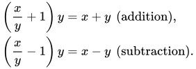
[edit]Addition and subtraction aren't typically performed on slide rules, but is possible using either of the following two techniques:[7]
- Converting addition and subtraction to division (required for the C and D or comparable scales):
- Exploits the identity that the quotient of two variables plus (or minus) one times the divisor equals their sum (or difference):
- This is similar to the addition/subtraction technique used for high-speed electronic circuits with a logarithmic number system in specialized computer applications like the Gravity Pipe (GRAPE) supercomputer and hidden Markov models.
- Using a linear L scale (available on some models):
- After sliding the cursor right (for addition) or left (for subtraction) and returning the slide to 0, the result can be read.
Generalizations
[edit]
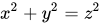
Using (almost) any strictly monotonic scales, other calculations can also be made with one movement.[8][9] For example, quadratic scales can be used to solve , used for instance by the Pythagorean theorem. Reciprocal scales can be used for the equality:which is useful for calculating parallel resistances, optical power, harmonic mean, etc.

Physical design
[edit]Standard linear rules
[edit]
The width of the slide rule is quoted in terms of the nominal width of the scales. Scales on the most common "10-inch" models are actually 25 cm, as they were made to metric standards, though some rules offer slightly extended scales to simplify manipulation when a result overflows. Pocket rules are typically 5 inches (12 cm). Models a couple of metres (yards) wide were made to be hung in classrooms for teaching purposes.[10]
Typically the divisions mark a scale to a precision of two significant figures, and the user estimates the third figure. Some high-end slide rules have magnifier cursors that make the markings easier to see. Such cursors can effectively double the accuracy of readings, permitting a 10-inch slide rule to serve as well as a 20-inch model.
Various other conveniences have been developed. Trigonometric scales are sometimes dual-labeled, in black and red, with complementary angles, the so-called "Darmstadt" style. Duplex slide rules often duplicate some of the scales on the back. Scales are often "split" to get higher accuracy. For example, instead of reading from an A scale to a D scale to find a square root, it may be possible to read from a D scale to an R1 scale running from 1 to square root of 10 or to an R2 scale running from square root of 10 to 10, where having more subdivisions marked can result in being able to read an answer with one more significant digit.
Circular slide rules
[edit] |
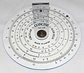
Circular slide rules come in two basic types, one with two cursors, and another with a free dish and one cursor. The dual cursor versions perform multiplication and division by holding a constant angle between the cursors as they are rotated around the dial. The onefold cursor version operates more like the standard slide rule through the appropriate alignment of the scales.
The basic advantage of a circular slide rule is that the widest dimension of the tool was reduced by a factor of about 3 (i.e. by π). For example, a 10 cm (3.9 in) circular would have a maximum precision approximately equal to a 31.4 cm (12.4 in) ordinary slide rule. Circular slide rules also eliminate "off-scale" calculations, because the scales were designed to "wrap around"; they never have to be reoriented when results are near 1.0—the rule is always on scale. However, for non-cyclical non-spiral scales such as S, T, and LL's, the scale width is narrowed to make room for end margins.[11]
Circular slide rules are mechanically more rugged and smoother-moving, but their scale alignment precision is sensitive to the centering of a central pivot; a minute 0.1 mm (0.0039 in) off-centre of the pivot can result in a 0.2 mm (0.0079 in) worst case alignment error. The pivot does prevent scratching of the face and cursors. The highest accuracy scales are placed on the outer rings. Rather than "split" scales, high-end circular rules use spiral scales for more complex operations like log-of-log scales. One eight-inch premium circular rule had a 50-inch spiral log-log scale. Around 1970, an inexpensive model from B. C. Boykin (Model 510) featured 20 scales, including 50-inch C-D (multiplication) and log scales. The RotaRule featured a friction brake for the cursor.
The main disadvantages of circular slide rules are the difficulty in locating figures along a dish, and limited number of scales. Another drawback of circular slide rules is that less-important scales are closer to the center, and have lower precisions. Most students learned slide rule use on the linear slide rules, and did not find reason to switch.
One slide rule remaining in daily use around the world is the E6-B. This is a circular slide rule first created in the 1930s for aircraft pilots to help with dead reckoning. With the aid of scales printed on the frame it also helps with such miscellaneous tasks as converting time, distance, speed, and temperature values, compass errors, and calculating fuel use. The so-called "prayer wheel" is still available in flight shops, and remains widely used. While GPS has reduced the use of dead reckoning for aerial navigation, and handheld calculators have taken over many of its functions, the E6-B remains widely used as a primary or backup device and the majority of flight schools demand that their students have some degree of proficiency in its use.
Proportion wheels are simple circular slide rules used in graphic design to calculate aspect ratios. Lining up the original and desired size values on the inner and outer wheels will display their ratio as a percentage in a small window. Though not as common since the advent of computerized layout, they are still made and used.[citation needed]
In 1952, Swiss watch company Breitling introduced a pilot's wristwatch with an integrated circular slide rule specialized for flight calculations: the Breitling Navitimer. The Navitimer circular rule, referred to by Breitling as a "navigation computer", featured airspeed, rate/time of climb/descent, flight time, distance, and fuel consumption functions, as well as kilometer—nautical mile and gallon—liter fuel amount conversion functions.
-
-
 A Russian circular slide rule built like a pocket watch that works as single cursor slide rule since the two needles are ganged together
 -
 A two-scale slide rule built into a ring
 -
 Pickett circular slide rule with two cursors. (4.25 in/10.9 cm width) Reverse has additional scale and one cursor.
 -
 Breitling Navitimer wristwatch with circular slide rule
 -
 The front side of a Boykin RotaRule Model 510
 -
 The rear side of a Boykin RotaRule Model 510
 -
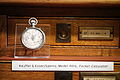 Pocket watch style Sperry 4016 Pocket Calculator
.jpg)


Cylindrical slide rules
[edit]Cylindrical slide rules are made in two styles: those with helical scales such as the Fuller calculator, the Otis King and the Bygrave slide rule, and those with bars, such as the Thacher and some Loga models. In either case, the advantage is a much longer scale, and hence potentially greater precision, than afforded by a straight or circular rule.
-
 Fuller calculator, 1928
 -
 Otis King Model K
 -
 Bygrave slide rule
 -
 Thacher slide rule, c. 1890

.jpg)


Materials
[edit]Traditionally slide rules were made out of a relatively dense, stable hardwood such as mahogany or boxwood with cursors of glass and metal. Aluminum was used, and at least one high precision instrument was made of steel.
In 1895, a Japanese firm, Hemmi, started to make slide rules from celluloid-clad bamboo, which had the advantages of being dimensionally stable, strong, and naturally self-lubricating. These bamboo slide rules were introduced in Sweden in September, 1933,[12] and probably only a little earlier in Germany.
Scales were also made of celluloid or other polymers, or printed on aluminium. Later cursors were molded from acrylics or polycarbonate, sometimes with Teflon bearing surfaces.
All premium slide rules had numbers and scales deeply engraved, and then filled with paint or other resin. Painted or imprinted slide rules were viewed as inferior, because the markings could wear off or be chemically damaged. Nevertheless, Pickett & Eckel, an American slide rule company, made only printed scale rules.[citation needed] Premium slide rules included clever mechanical catches so the rule would not fall apart by accident, and bumpers to protect the scales and cursor from rubbing on tabletops.
History
[edit]

The slide rule was invented around 1620–1630, shortly after John Napier's publication of the concept of the logarithm. In 1620 Edmund Gunter of Oxford developed a calculating device with a single logarithmic scale; with additional measuring tools it could be used to multiply and divide.[13] In c. 1622, William Oughtred of Cambridge combined two handheld Gunter rules to make a device that is recognizably the modern slide rule.[14] Oughtred became involved in a vitriolic controversy over priority, with his one-time student Richard Delamain and the prior claims of Edmund Wingate. Oughtred's ideas were only made public in publications of his student William Forster in 1632 and 1653.
In 1677, Henry Coggeshall created a two-foot folding rule for timber measure, called the Coggeshall slide rule, expanding the slide rule's use beyond mathematical inquiry.
In 1722, Warner introduced the two- and three-decade scales, and in 1755 Everard included an inverted scale; a slide rule containing all of these scales is usually known as a "polyphase" rule.
In 1815, Peter Mark Roget invented the log log slide rule, which included a scale displaying the logarithm of the logarithm. This allowed the user to directly perform calculations involving roots and exponents. This was especially useful for fractional powers.
In 1821, Nathaniel Bowditch, described in the American Practical Navigator a "sliding rule" that contained scaled trigonometric functions on the fixed part and a line of log-sines and log-tans on the slider used to solve navigation problems.
In 1845, Paul Cameron of Glasgow introduced a nautical slide rule capable of answering navigation questions, including right ascension and declination of the sun and principal stars.[15]
Modern form
[edit]
A more modern form of slide rule was created in 1859 by French artillery lieutenant Amédée Mannheim, who was fortunate both in having his rule made by a firm of national reputation, and its adoption by the French Artillery. Mannheim's rule had two major modifications that made it easier to use than previous general-purpose slide rules. Such rules had four basic scales, A, B, C, and D, and D was the only single-decade logarithmic scale; C had two decades, like A and B. Most operations were done on the A and B scales; D was only used for finding squares and square roots.
Mannheim changed the C scale to a single-decade scale and performed most operations with C and D instead of A and B. Because the C and D scales were single-decade, they could be read more precisely, so the rule's results could be more accurate. The change also made it easier to include squares and square roots as part of a larger calculation. Mannheim's rule also had a cursor, unlike almost all preceding rules, so any of the scales could be easily and accurately compared across the rule width. The "Mannheim rule" became the standard slide rule arrangement for the later 19th century and remained a common standard throughout the slide-rule era.
The growth of the engineering profession during the later 19th century drove widespread slide-rule use, beginning in Europe and eventually taking hold in the United States as well. The duplex rule was invented by William Cox in 1891 and was produced by Keuffel and Esser Co. of New York.[16][17]
In 1881, the American inventor Edwin Thacher introduced his cylindrical rule, which had a much longer scale than standard linear rules and thus could calculate to higher precision, about four to five significant digits. However, the Thacher rule was quite expensive, as well as being non-portable, so it was used in far more limited numbers than conventional slide rules.
Astronomical work also required precise computations, and, in 19th-century Germany, a steel slide rule about two meters long was used at one observatory. It had a microscope attached, giving it accuracy to six decimal places.[citation needed]
20th century
[edit]
In the 1920s, the novelist and engineer Nevil Shute Norway (he called his autobiography Slide Rule) was Chief Calculator on the design of the British R100 airship for Vickers Ltd. from 1924. The stress calculations for each transverse frame required computations by a pair of calculators (people) using Fuller's cylindrical slide rules for two or three months. The simultaneous equation contained up to seven unknown quantities, took about a week to solve, and had to be repeated with a different selection of slack wires if the guess on which of the eight radial wires were slack was wrong and one of the wires guessed to be slack was not slack. After months of labour filling perhaps fifty foolscap sheets with calculations "the truth stood revealed (and) produced a satisfaction almost amounting to a religious experience".[18]
In 1937, physicist Lucy Hayner designed and constructed a circular slide rule in Braille.[19]
Throughout the 1950s and 1960s, the slide rule was the symbol of the engineer's profession in the same way the stethoscope is that of the medical profession.[20]
Aluminium Pickett-brand slide rules were carried on Project Apollo space missions. The model N600-ES owned by Buzz Aldrin that flew with him to the Moon on Apollo 11 was sold at auction in 2007.[21] The model N600-ES taken along on Apollo 13 in 1970 is owned by the National Air and Space Museum.[22]
Some engineering students and engineers carried ten-inch slide rules in belt holsters, a common sight on campuses even into the mid-1970s. Until the advent of the pocket digital calculator, students also might keep a ten- or twenty-inch rule for precision work at home or the office[23] while carrying a five-inch pocket slide rule around with them.
In 2004, education researchers David B. Sher and Dean C. Nataro conceived a new type of slide rule based on prosthaphaeresis, an algorithm for rapidly computing products that predates logarithms. However, there has been little practical interest in constructing one beyond the initial prototype.[24]
Specialized calculators
[edit]Slide rules have often been specialized to varying degrees for their field of use, such as excise, proof calculation, engineering, navigation, etc., and some slide rules are extremely specialized for very narrow applications. For example, the John Rabone & Sons 1892 catalog lists a "Measuring Tape and Cattle Gauge", a device to estimate the weight of a cow from its measurements.
There were many specialized slide rules for photographic applications. For example, the actinograph of Hurter and Driffield was a two-slide boxwood, brass, and cardboard device for estimating exposure from time of day, time of year, and latitude.
Specialized slide rules were invented for various forms of engineering, business and banking. These often had common calculations directly expressed as special scales, for example loan calculations, optimal purchase quantities, or particular engineering equations. For example, the Fisher Controls company distributed a customized slide rule adapted to solving the equations used for selecting the proper size of industrial flow control valves.[25]
Pilot balloon slide rules were used by meteorologists in weather services to determine the upper wind velocities from an ascending hydrogen or helium-filled pilot balloon.[26]
The E6-B is a circular slide rule used by pilots and navigators.
Circular slide rules to estimate ovulation dates and fertility are known as wheel calculators.[27]
A Department of Defense publication from 1962[28] infamously included a special-purpose circular slide rule for calculating blast effects, overpressure, and radiation exposure from a given yield of an atomic bomb.[29]
-
 An E6-B aviation computer
 -
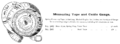 John Rabone & Sons 1892 cattle gauge
 -

-
 Cryptographic slide rule used by the Swiss Army between 1914 and 1940
 -
 Rare fractional adder


Decline
[edit]
The importance of the slide rule began to diminish as electronic computers, a new but rare resource in the 1950s, became more widely available to technical workers during the 1960s.
The first step away from slide rules was the introduction of relatively inexpensive electronic desktop scientific calculators. These included the Wang Laboratories LOCI-2,[30][31] introduced in 1965, which used logarithms for multiplication and division; and the Hewlett-Packard HP 9100A, introduced in 1968.[32] Both of these were programmable and provided exponential and logarithmic functions; the HP had trigonometric functions (sine, cosine, and tangent) and hyperbolic trigonometric functions as well. The HP used the CORDIC (coordinate rotation digital computer) algorithm,[33] which allows for calculation of trigonometric functions using only shift and add operations. This method facilitated the development of ever smaller scientific calculators.
As with mainframe computing, the availability of these desktop machines did not significantly affect the ubiquitous use of the slide rule, until cheap hand-held scientific electronic calculators became available in the mid-1970s, at which point it rapidly declined. The pocket-sized Hewlett-Packard HP-35 scientific calculator was the first handheld device of its type, but it cost US$395 in 1972. This was justifiable for some engineering professionals, but too expensive for most students.
Around 1974, lower-cost handheld electronic scientific calculators started to make slide rules largely obsolete.[34][35][36][37] By 1975, basic four-function electronic calculators could be purchased for less than $50, and by 1976 the TI-30 scientific calculator was sold for less than $25 ($138 adjusted for inflation).
1980 was the final year of the University Interscholastic League (UIL) competition in Texas to use slide rules. The UIL had been originally been organized in 1910 to administer literary events, but had become the governing body of school sports events as well.[38]
Comparison to electronic digital calculators
[edit]
Even during their heyday, slide rules never caught on with the general public.[39] Addition and subtraction are not well-supported operations on slide rules and doing a calculation on a slide rule tends to be slower than on a calculator.[40] This led engineers to use mathematical equations that favored operations that were easy on a slide rule over more accurate but complex functions; these approximations could lead to inaccuracies and mistakes.[41] On the other hand, the spatial, manual operation of slide rules cultivates in the user an intuition for numerical relationships and scale that people who have used only digital calculators often lack.[42] A slide rule will also display all the terms of a calculation along with the result, thus eliminating uncertainty about what calculation was actually performed. It has thus been compared with reverse Polish notation (RPN) implemented in electronic calculators.[43]
A slide rule requires the user to separately compute the order of magnitude of the answer to position the decimal point in the results. For example, 1.5 × 30 (which equals 45) will show the same result as 1500000 × 0.03 (which equals 45000). This separate calculation forces the user to keep track of magnitude in short-term memory (which is error-prone), keep notes (which is cumbersome) or reason about it in every step (which distracts from the other calculation requirements).
The typical arithmetic precision of a slide rule is about three significant digits, compared to many digits on digital calculators. As order of magnitude gets the greatest prominence when using a slide rule, users are less likely to make errors of false precision.
When performing a sequence of multiplications or divisions by the same number, the answer can often be determined by merely glancing at the slide rule without any manipulation. This can be especially useful when calculating percentages (e.g. for test scores) or when comparing prices (e.g. in dollars per kilogram). Multiple speed-time-distance calculations can be performed hands-free at a glance with a slide rule. Other useful linear conversions such as pounds to kilograms can be easily marked on the rule and used directly in calculations.
Being entirely mechanical, a slide rule does not depend on grid electricity or batteries. Mechanical imprecision in slide rules that were poorly constructed or warped by heat or use will lead to errors.
Many sailors keep slide rules as backups for navigation in case of electric failure or battery depletion on long route segments. Slide rules are still commonly used in aviation, particularly for smaller planes. They are being replaced only by integrated, special purpose and expensive flight computers, and not general-purpose calculators. The E6-B circular slide rule used by pilots has been in continuous production and remains available in a variety of models. Some wrist watches designed for aviation use still feature slide rule scales to permit quick calculations. The Citizen Skyhawk AT and the Seiko Flightmaster SNA411 are two notable examples.[44]
Contemporary use
[edit] | This section possibly contains original research. (February 2015) |

Even in the 21st century, some people prefer a slide rule over an electronic calculator as a practical computing device. Others keep their old slide rules out of a sense of nostalgia, or collect them as a hobby.[45]
A popular collectible model is the Keuffel & Esser Deci-Lon, a premium scientific and engineering slide rule available both in a ten-inch (25 cm) "regular" (Deci-Lon 10) and a five-inch "pocket" (Deci-Lon 5) variant. Another prized American model is the eight-inch (20 cm) Scientific Instruments circular rule. Of European rules, Faber-Castell's high-end models are the most popular among collectors.
Although a great many slide rules are circulating on the market, specimens in good condition tend to be expensive. Many rules found for sale on online auction sites are damaged or have missing parts, and the seller may not know enough to supply the relevant information. Replacement parts are scarce, expensive, and generally available only for separate purchase on individual collectors' web sites. The Keuffel and Esser rules from the period up to about 1950 are particularly problematic, because the end-pieces on the cursors, made of celluloid, tend to chemically break down over time. Methods of preserving plastic may be used to slow the deterioration of some older slide rules, and 3D printing may be used to recreate missing or irretrievably broken cursor parts.[46]
There are still a handful of sources for brand new slide rules. The Concise Company of Tokyo, which began as a manufacturer of circular slide rules in July 1954,[47] continues to make and sell them today. In September 2009, on-line retailer ThinkGeek introduced its own brand of straight slide rules, described as "faithful replica[s]" that were "individually hand tooled".[48] These were no longer available in 2012.[49] In addition, Faber-Castell had a number of slide rules in inventory, available for international purchase through their web store, until mid 2018.[50] Proportion wheels are still used in graphic design.
Various slide rule simulator apps are available for Android and iOS-based smart phones and tablets.
Specialized slide rules such as the E6-B used in aviation, and gunnery slide rules used in laying artillery are still used though no longer on a routine basis. These rules are used as part of the teaching and instruction process as in learning to use them the student also learns about the principles behind the calculations, it also allows the student to be able to use these instruments as a backup in the event that the modern electronics in general use fail.
Collections
[edit]
The MIT Museum in Cambridge, Massachusetts, has a collection of hundreds of slide rules, nomograms, and mechanical calculators.[51] The Keuffel and Esser Company collection, from the slide rule manufacturer formerly located in Hoboken, New Jersey, was donated to MIT around 2005, substantially expanding existing holdings.[52] Selected items from the collection are usually on display at the museum.[53][54]
The International Slide Rule Museum is claimed to be "[the world's] most extensive resource for all things concerning slide rules and logarithmic calculators".[55] The museum's Web page includes extensive literature relative to slide rules in its "Slide Rule Library" section.[56]
See also
[edit]- Abacus – Calculating tool
- Computer (occupation) – Person performing mathematical calculations, before electronic calculators
- Curta – Mechanical pocket calculator
- Flight computer – Circular slide rule used in aviation
- Floating point – Computer approximation for real numbers
- Hans Peter Luhn – American computer scientist
- Nomogram – Analog graphical calculator
- Sector (instrument) – Mathematical instrument consisting of two hinged rulers
- Slide calculator – Mechanical calculator
- Slide chart
- Timeline of computing
- Vernier scale – Auxiliary scale of a measurement device, used to increase precision
- Volvelle – Paper construct with rotating parts
References
[edit]- ^ Roger R. Flynn (June 2002). Computer sciences. Vol. 1. Macmillan. p. 175. ISBN 978-0-02-865567-3. Retrieved 2013-03-30.
The slide rule is an example of a mechanical analog computer...
- ^ Ernst Bleuler; Robert Ozias Haxby (2011-09-21). Electronic Methods. Academic Press. p. 638. ISBN 978-0-08-085975-0. Retrieved 2013-03-30.
For example, slide rules are mechanical analog computers
- ^ "Slide Rules". MIT Museum. Massachusetts Institute of Technology. Retrieved 2019-05-01.
- ^ Berrey, Lester V.; van den Bark, Melvin (1953). American Thesaurus of Slang: A Complete Reference Book of Colloquial Speech (2nd ed.). Crowell. OCLC 319462.
- ^ Petroski, Henry (2011). An Engineer's Alphabet: Gleanings from the Softer Side of a Profession. Cambridge University Press. pp. 46–47. ISBN 9781139505307. Retrieved 2017-03-21.
- ^ Marcotte, Ph.D., Eric (2002). "Eric's Types of Slide Rules and their Scales". www.sliderule.ca. Retrieved 2021-07-13.
- ^ "AntiQuark: Slide Rule Tricks". antiquark.com.
- ^ Istvan, Szalkai (2016). "General Two-Variable Functions on the Slide Rule". Journal of the Oughtred Society. 27 (1): 14–18. arXiv:1612.03955.
- ^ Istvan, Szalkai (2016). "General Two-variable Functions on the Slide-rule". arXiv:1612.03955 [math.HO].
- ^ "Slide Rules". Tbullock.com. 2009-12-08. Archived from the original on 2013-02-03. Retrieved 2010-02-20.
- ^ At least one circular rule, a 1931 Gilson model, sacrificed some of the scales usually found in slide rules in order to obtain additional resolution in multiplication and division. It functioned through the use of a spiral C scale, which was claimed to be 50 feet and readable to five significant figures. See http://www.sphere.bc.ca/test/gilson/gilson-manual2.jpg Archived 2006-12-30 at the Wayback Machine. A photo can be seen at https://www.hpmuseum.org/srcirc.htm. An instruction manual for the unit marketed by Dietzgen can be found at http://www.sliderulemuseum.com/SR_Library_General.htm Archived 2007-02-14 at the Wayback Machine. All retrieved March 14, 2007.
- ^ "336 (Teknisk Tidskrift / 1933. Allmänna avdelningen)". Runeberg.org. Retrieved 2010-02-20.
- ^ Smith, David E. (1958). History of Mathematics. Courier Corporation. p. 205. ISBN 9780486204307.
{{cite book}}: ISBN / Date incompatibility (help) - ^ Applebaum, Wilbur (2003-12-16). "Slide Rule". Encyclopedia of the Scientific Revolution: From Copernicus to Newton. Routledge. ISBN 9781135582555.
- ^ "Cameron's Nautical Slide Rule", The Practical Mechanic and Engineer's Magazine, April 1845, p. 187 and Plate XX-B
- ^ Kells, Lyman M.; Kern, Willis F.; Bland, James R. (1943). The Log-Log Duplex Decitrig Slide Rule No. 4081: A Manual. Keuffel & Esser. p. 92. Archived from the original on 2009-02-14.
- ^ The Polyphase Duplex Slide Rule, A Self-Teaching Manual, Breckenridge, 1922, p. 20.
- ^ Norway, Nevil Shute (1954). Slide Rule. London: William Heinemann. pp. 76–78.
- ^ Witcher, C. M. (1954-12-01). "Physics without sight". Physics Today. 7 (12): 8–10. Bibcode:1954PhT.....7l...8W. doi:10.1063/1.3061483.
- ^ Stoll, Cliff (2006). "When Slide Rules Ruled". Scientific American. 294 (5): 80–87. Bibcode:2006SciAm.294e..80S. doi:10.1038/scientificamerican0506-80. JSTOR 26061456. PMID 16708492.
- ^ "Lot 25368 Buzz Aldrin's Apollo 11 Slide Rule – Flown to the Moon. ... 2007 September Grand Format Air & Space Auction #669". Heritage Auctions. Archived from the original on 2013-09-03. Retrieved 2013-09-03.
- ^ "Slide Rule, 5-inch, Pickett N600-ES, Apollo 13". Smithsonian National Air and Space Museum. Archived from the original on 2013-10-09. Retrieved 2013-09-03.
- ^ Charles Overton Harris, Slide rule simplified, American Technical Society, 1961, p. 5.
- ^ Sher, David B.; Nataro, Dean C. (2009-06-02). "The Prosthaphaeretic Slide Rule: A Mechanical Multiplication Device Based On Trigonometric Identities". Mathematics And Computer Education, Vol. 38, Iss. 1 (Winter 2004): 37–43. Archived from the original on 2005-05-10. Retrieved 2010-02-20 – via Findarticles.com.
- ^ "Fisher sizing rules". natgasedu.com. Archived from the original on 2010-01-06. Retrieved 2009-10-06.
- ^ "Pilot Balloon Slide Rules". www.pilotballoon.com. Archived from the original on 2016-09-28. Retrieved 2016-09-28.
- ^ Ross, M. G. (2003). "Circle of time: errors in the use of the pregnancy wheel". Journal of Maternal-Fetal and Neonatal Medicine. 14 (6): 370–372. doi:10.1080/14767050412331312200. PMID 15061314.
- ^ "The Effects of Nuclear Weapons". Retrieved 2021-05-02.
- ^ "Strangelove Slide Rule". Retrieved 2021-05-02.
- ^ "The Wang LOCI-2". oldcalculatormuseum.com.
- ^ Wang Laboratories (December 1966). "Now you can determine Copolymer Composition in a few minutes at your desk". Analytical Chemistry. 38 (13): 62A – 63A. doi:10.1021/ac50155a005.
- ^ Leibson, Steven (2010). "The HP 9100 Project: An Exothermic Reaction". Retrieved 2024-06-16.
- ^ Volder, Jack E. (June 2000). "The Birth of CORDIC" (PDF). Journal of VLSI Signal Processing. 25 (2): 101–105. Bibcode:2000JSPSy..25..101V. doi:10.1023/a:1008110704586. ISSN 0922-5773. Archived from the original (PDF) on 2016-03-04. Retrieved 2016-01-02.
- ^ Behrens, Lawrence; Rosen, Leonard J. (1982). Writing and reading across the curriculum. Little, Brown. p. 273.
Then, just a decade ago, the invention of the pocket calculator made the slide rule obsolete almost overnight...
- ^ Maor, Eli (2009). e: The Story of a Number. Princeton University Press. p. 16. ISBN 978-0-691-14134-3.
Then in the early 1970s the first electronic hand-held calculators appeared on the market, and within ten years the slide rule was obsolete.
- ^ Castleden, Rodney (2007). Inventions that Changed the World. Futura. p. 157. ISBN 978-0-7088-0786-6.
With the invention of the calculator the slide rule became instantly obsolete.
- ^ Denning, Peter J.; Metcalfe, Robert M. (1998). Beyond calculation: the next fifty years of computing. Springer. p. xiv. ISBN 978-0-387-98588-6.
The first hand calculator appeared in 1972 and made the slide rule obsolete overnight.
- ^ Gabbert, Mike (Fall 1999). "Slide Rule Competition in Texas High Schools" (PDF). Journal of the Oughtred Society. 8 (2): 56–58. Retrieved 2025-03-05.
- ^ Stoll, Cliff. "When Slide Rules Ruled," Scientific American, May 2006, pp. 80–87. "The difficulty of learning to use slide rules discouraged their use among the hoi polloi. Yes, the occasional grocery store manager figured discounts on a slipstick, and this author once caught his high school English teacher calculating stats for trifecta horse-race winners on a slide rule during study hall. But slide rules never made it into daily life because you could not do simple addition and subtraction with them, not to mention the difficulty of keeping track of the decimal point. Slide rules remained tools for techies."
- ^ Watson, George H. "Problem-based learning and the three C's of technology," The Power of Problem-Based Learning, Barbara Duch, Susan Groh, Deborah Allen, eds., Stylus Publishing, LLC, 2001. "Numerical computations in freshman physics and chemistry were excruciating; however, this did not seem to be the case for those students fortunate enough to already own a calculator. I vividly recall that at the end of 1974, the students who were still using slide rules were given an additional 15 minutes on the final examination to compensate for the computational advantage afforded by the calculator, hardly adequate compensation in the opinions of the remaining slide rule practitioners."
- ^ Stoll, Cliff. "When Slide Rules Ruled," Scientific American, May 2006, pp. 80–87. "With computation moving literally at a hand's pace and the lack of precision a given, mathematicians worked to simplify complex problems. Because linear equations were friendlier to slide rules than more complex functions were, scientists struggled to linearize mathematical relations, often sweeping high-order or less significant terms under the computational carpet. So a car designer might calculate gas consumption by looking mainly at an engine's power, while ignoring how air friction varies with speed. Engineers developed shortcuts and rules of thumb. At their best, these measures led to time savings, insight and understanding. On the downside, these approximations could hide mistakes and lead to gross errors."
- ^ Stoll, Cliff. "When Slide Rules Ruled", Scientific American, May 2006, pp. 80–87. "One effect was that users felt close to the numbers, aware of rounding-off errors and systematic inaccuracies, unlike users of today's computer-design programs. Chat with an engineer from the 1950s, and you will most likely hear a lament for the days when calculation went hand-in-hand with deeper comprehension. Instead of plugging numbers into a computer program, an engineer would understand the fine points of loads and stresses, voltages and currents, angles and distances. Numeric answers, crafted by hand, meant problem solving through knowledge and analysis rather than sheer number crunching."
- ^ Williams, Al (2023-06-21). "In Praise Of RPN (with Python Or C)". Hackaday. Archived from the original on 2023-09-23. Retrieved 2023-09-23.
- ^ "Citizen Watch Company – Citizen Eco-Drive / US, Canada, UK, IrelandCitizen Watch". citizenwatch.com. Archived from the original on 2014-04-22. Retrieved 2014-04-21.
- ^ "Greg's Slide Rules – Links to Slide Rule Collectors". Sliderule.ozmanor.com. 2004-07-29. Retrieved 2010-02-20.
- ^ "Restoring and Repairing Slide Rules and Notes". International Slide Rule Museum.
- ^ "About CONCISE". Concise.co.jp. Archived from the original on 2012-03-12. Retrieved 2010-02-20.
- ^ "Slide Rule". ThinkGeek. Archived from the original on 2010-03-27. Retrieved 2015-04-08.
- ^ "Slide Rule". ThinkGeek. Archived from the original on 2012-04-15. Retrieved 2015-04-08.
- ^ "Rechenschieber". Faber-Castell. Archived from the original on 2013-11-21. Retrieved 2012-01-17. It is believed they may still have some slide rules, but their new website and online store does not carry them.
- ^ "Commons category MIT Slide Rule Collection".
- ^ "MIT Museum measures up". MIT News. Massachusetts Institute of Technology. 2005-01-11. Retrieved 2019-05-01.
- ^ "Slide Rules". MIT Museum. Massachusetts Institute of Technology. Archived from the original on 2019-05-01. Retrieved 2019-05-01.
- ^ "MIT Museum — Slide Rules". proundesign.com. Proun Design. Archived from the original on 2019-05-01. Retrieved 2019-05-01.
- ^ Turner, Kimberli (2009-10-07). "Slide Rule: 101". Colorado Hometown Newspapers.
- ^ "Slide Rule Library Main Desk". International Slide Rule Museum. Archived from the original on 2023-01-07. Retrieved 2023-01-07.
External links
[edit]
- International Slide Rule Museum
- The history, theory and use of the engineering slide rule — By Dr James B. Calvert, University of Denver
- United Kingdom Slide Rule Circle Home Page Archived 2015-09-28 at the Wayback Machine
- Oughtred Society Slide Rule Home Page — Dedicated to the preservation and history of slide rules
- Rod Lovett's Slide Rules – Comprehensive Aristo site with many search facilities
- Derek's virtual slide rule gallery — Javascript simulations of historical slide rules
- . New International Encyclopedia. 1905.
- . Encyclopedia Americana. 1920.
- Reglas de Cálculo — A very big Faber Castell collection
- Collection of slide rules — French Slide Rules (Graphoplex, Tavernier-Gravet and others)
- Eric's Slide Rule Site — History and use
- Slide Rules — Information from The Museum of HP Calculators
- Descriptions, alphabetical by brandname, with images (Vintage Tech. Assoc.)
- On the History of Gunter's Scale and the Slide Rule During the Seventeenth Century at Project Gutenberg
- The Slide Rule: a Practical Manual at Project Gutenberg
Calculator | |||||||||||||
|---|---|---|---|---|---|---|---|---|---|---|---|---|---|
| Manual | |||||||||||||
| Logarithm |
| ||||||||||||
| Mechanical |
| ||||||||||||
| Electronic |
| ||||||||||||
| Software | |||||||||||||
| Historical | |||||||||||||


| International | |
|---|---|
| National | |
| Other | |