Hubbry Logo
search
logo

S-matrix

logo
Community Hub0 Subscribers
Read side by side
from Wikipedia

In physics, the S-matrix or scattering matrix is a matrix that relates the initial state and the final state of a physical system undergoing a scattering process. It is used in quantum mechanics, scattering theory and quantum field theory (QFT).

More formally, in the context of QFT, the S-matrix is defined as the unitary matrix connecting sets of asymptotically free particle states (the in-states and the out-states) in the Hilbert space of physical states: a multi-particle state is said to be free (or non-interacting) if it transforms under Lorentz transformations as a tensor product, or direct product in physics parlance, of one-particle states as prescribed by equation (1) below. Asymptotically free then means that the state has this appearance in either the distant past or the distant future.

While the S-matrix may be defined for any background (spacetime) that is asymptotically solvable and has no event horizons, it has a simple form in the case of the Minkowski space. In this special case, the Hilbert space is a space of irreducible unitary representations of the inhomogeneous Lorentz group (the Poincaré group); the S-matrix is the evolution operator between (the distant past), and (the distant future). It is defined only in the limit of zero energy density (or infinite particle separation distance).

It can be shown that if a quantum field theory in Minkowski space has a mass gap, the state in the asymptotic past and in the asymptotic future are both described by Fock spaces.

History

[edit]

The initial elements of S-matrix theory are found in Paul Dirac's 1927 paper "Über die Quantenmechanik der Stoßvorgänge".[1][2] The S-matrix was first properly introduced by John Archibald Wheeler in the 1937 paper "On the Mathematical Description of Light Nuclei by the Method of Resonating Group Structure".[3] In this paper Wheeler introduced a scattering matrix – a unitary matrix of coefficients connecting "the asymptotic behaviour of an arbitrary particular solution [of the integral equations] with that of solutions of a standard form",[4] but did not develop it fully.

In the 1940s, Werner Heisenberg independently developed and substantiated the idea of the S-matrix. Because of the problematic divergences present in quantum field theory at that time, Heisenberg was motivated to isolate the essential features of the theory that would not be affected by future changes as the theory developed. In doing so, he was led to introduce a unitary "characteristic" S-matrix.[4]

Today, however, exact S-matrix results are important for conformal field theory, integrable systems, and several further areas of quantum field theory and string theory. S-matrices are not substitutes for a field-theoretic treatment, but rather, complement the end results of such.

Motivation

[edit]

In high-energy particle physics one is interested in computing the probability for different outcomes in scattering experiments. These experiments can be broken down into three stages:

  1. Making a collection of incoming particles collide (usually two kinds of particles with high energies).
  2. Allowing the incoming particles to interact. These interactions may change the types of particles present (e.g. if an electron and a positron annihilate they may produce two photons).
  3. Measuring the resulting outgoing particles.

The process by which the incoming particles are transformed (through their interaction) into the outgoing particles is called scattering. For particle physics, a physical theory of these processes must be able to compute the probability for different outgoing particles when different incoming particles collide with different energies.

The S-matrix in quantum field theory achieves exactly this. It is assumed that the small-energy-density approximation is valid in these cases.

Use

[edit]

The S-matrix is closely related to the transition probability amplitude in quantum mechanics and to cross sections of various interactions; the elements (individual numerical entries) in the S-matrix are known as scattering amplitudes. Poles of the S-matrix in the complex-energy plane are identified with bound states, virtual states or resonances. Branch cuts of the S-matrix in the complex-energy plane are associated to the opening of a scattering channel.

In the Hamiltonian approach to quantum field theory, the S-matrix may be calculated as a time-ordered exponential of the integrated Hamiltonian in the interaction picture; it may also be expressed using Feynman's path integrals. In both cases, the perturbative calculation of the S-matrix leads to Feynman diagrams.

In scattering theory, the S-matrix is an operator mapping free particle in-states to free particle out-states (scattering channels) in the Heisenberg picture. This is very useful because often we cannot describe the interaction (at least, not the most interesting ones) exactly.

In one-dimensional quantum mechanics

[edit]

A simple prototype in which the S-matrix is 2-dimensional is considered first, for the purposes of illustration. In it, particles with sharp energy E scatter from a localized potential V according to the rules of 1-dimensional quantum mechanics. Already this simple model displays some features of more general cases, but is easier to handle.

Each energy E yields a matrix S = S(E) that depends on V. Thus, the total S-matrix could, figuratively speaking, be visualized, in a suitable basis, as a "continuous matrix" with every element zero except for 2 × 2-blocks along the diagonal for a given V.

Definition

[edit]

Consider a localized one dimensional potential barrier V(x), subjected to a beam of quantum particles with energy E. These particles are incident on the potential barrier from left to right.

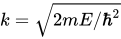
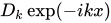
The solutions of the Schrödinger equation outside the potential barrier are plane waves given by for the region to the left of the potential barrier, and for the region to the right to the potential barrier, where is the wave vector. The time dependence is not needed in our overview and is hence omitted. The term with coefficient A represents the incoming wave, whereas term with coefficient C represents the outgoing wave. B stands for the reflecting wave. Since we set the incoming wave moving in the positive direction (coming from the left), D is zero and can be omitted.


The "scattering amplitude", i.e., the transition overlap of the outgoing waves with the incoming waves is a linear relation defining the S-matrix,
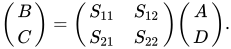
The above relation can be written as where The elements of S completely characterize the scattering properties of the potential barrier V(x).


Unitary property

[edit]

The unitary property of the S-matrix is directly related to the conservation of the probability current in quantum mechanics.

The probability current density J of the wave function ψ(x) is defined as The probability current density of to the left of the barrier is while the probability current density of to the right of the barrier is
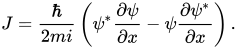
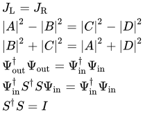
For conservation of the probability current, JL = JR. This implies the S-matrix is a unitary matrix.

Proof

Time-reversal symmetry

[edit]

If the potential V(x) is real, then the system possesses time-reversal symmetry. Under this condition, if ψ(x) is a solution of the Schrödinger equation, then ψ*(x) is also a solution.

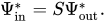
The time-reversed solution is given by for the region to the left to the potential barrier, and for the region to the right to the potential barrier, where the terms with coefficient B*, C* represent incoming wave, and terms with coefficient A*, D* represent outgoing wave.


They are again related by the S-matrix, that is,
Now, the relations together yield a condition This condition, in conjunction with the unitarity relation, implies that the S-matrix is symmetric, as a result of time reversal symmetry,

By combining the symmetry and the unitarity, the S-matrix can be expressed in the form: with and . So the S-matrix is determined by three real parameters.

Transfer matrix

[edit]

The transfer matrix relates the plane waves and on the right side of scattering potential to the plane waves and on the left side:[5]

and its components can be derived from the components of the S-matrix via:[6] and , whereby time-reversal symmetry is assumed.
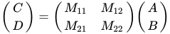

In the case of time-reversal symmetry, the transfer matrix can be expressed by three real parameters:

with and (in case r = 1 there would be no connection between the left and the right side)

Finite square well

[edit]

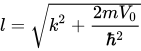
The one-dimensional, non-relativistic problem with time-reversal symmetry of a particle with mass m that approaches a (static) finite square well, has the potential function V with The scattering can be solved by decomposing the wave packet of the free particle into plane waves with wave numbers for a plane wave coming (faraway) from the left side or likewise (faraway) from the right side.

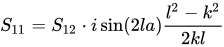
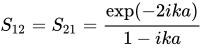
The S-matrix for the plane wave with wave number k has the solution:[6] and  ; hence and therefore and in this case.
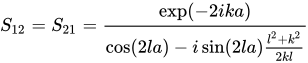
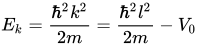
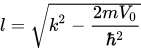
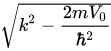
Whereby is the (increased) wave number of the plane wave inside the square well, as the energy eigenvalue associated with the plane wave has to stay constant:
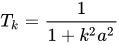
The transmission is

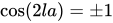
In the case of then and therefore and i.e. a plane wave with wave number k passes the well without reflection if for a

Finite square barrier

[edit]

The square barrier is similar to the square well with the difference that for .

There are three different cases depending on the energy eigenvalue of the plane waves (with wave numbers k resp. k) far away from the barrier:

  • : In this case and the formulas for have the same form as is in the square well case, and the transmission is
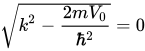
  • : In this case and the wave function has the property inside the barrier and

    and

    The transmission is: . This intermediate case is not singular, it's the limit ( resp. ) from both sides.
  • :In this case is an imaginary number. So the wave function inside the barrier has the components and with .

    The solution for the S-matrix is:[7]

    and likewise: and also in this case .

    The transmission is .

Transmission coefficient and reflection coefficient

[edit]

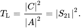
The transmission coefficient from the left of the potential barrier is, when D = 0,
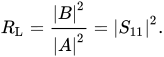
The reflection coefficient from the left of the potential barrier is, when D = 0,
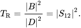
Similarly, the transmission coefficient from the right of the potential barrier is, when A = 0,
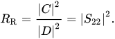
The reflection coefficient from the right of the potential barrier is, when A = 0,
The relations between the transmission and reflection coefficients are and This identity is a consequence of the unitarity property of the S-matrix.


With time-reversal symmetry, the S-matrix is symmetric and hence and .

Optical theorem in one dimension

[edit]

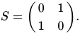
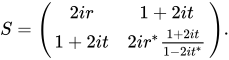
In the case of free particles V(x) = 0, the S-matrix is[8] Whenever V(x) is different from zero, however, there is a departure of the S-matrix from the above form, to This departure is parameterized by two complex functions of energy, r and t. From unitarity there also follows a relationship between these two functions,
The analogue of this identity in three dimensions is known as the optical theorem.

Definition in quantum field theory

[edit]

Interaction picture

[edit]

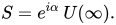
A straightforward way to define the S-matrix begins with considering the interaction picture.[9] Let the Hamiltonian H be split into the free part H0 and the interaction V, H = H0 + V. In this picture, the operators behave as free field operators and the state vectors have dynamics according to the interaction V. Let denote a state that has evolved from a free initial state The S-matrix element is then defined as the projection of this state on the final state Thus where S is the S-operator. The great advantage of this definition is that the time-evolution operator U evolving a state in the interaction picture is formally known,[10] where T denotes the time-ordered product. Expressed in this operator, from which Expanding using the knowledge about U gives a Dyson series, or, if V comes as a Hamiltonian density ,

Being a special type of time-evolution operator, S is unitary. For any initial state and any final state one finds

This approach is somewhat naïve in that potential problems are swept under the carpet.[11] This is intentional. The approach works in practice and some of the technical issues are addressed in the other sections.

In and out states

[edit]

Here a slightly more rigorous approach is taken in order to address potential problems that were disregarded in the interaction picture approach of above. The final outcome is, of course, the same as when taking the quicker route. For this, the notions of in and out states are needed. These will be developed in two ways, from vacuum, and from free particle states. Needless to say, the two approaches are equivalent, but they illuminate matters from different angles.

From vacuum

[edit]

If a(k) is a creation operator, its hermitian adjoint is an annihilation operator and destroys the vacuum,

In Dirac notation, define as a vacuum quantum state, i.e. a state without real particles. The asterisk signifies that not all vacua are necessarily equal, and certainly not equal to the Hilbert space zero state 0. All vacuum states are assumed Poincaré invariant, invariance under translations, rotations and boosts,[11] formally, where Pμ is the generator of translation in space and time, and Mμν is the generator of Lorentz transformations. Thus the description of the vacuum is independent of the frame of reference. Associated to the in and out states to be defined are the in and out field operators (aka fields) Φi and Φo. Attention is here focused to the simplest case, that of a scalar theory in order to exemplify with the least possible cluttering of the notation. The in and out fields satisfy the free Klein–Gordon equation. These fields are postulated to have the same equal time commutation relations (ETCR) as the free fields, where πi,j is the field canonically conjugate to Φi,j. Associated to the in and out fields are two sets of creation and annihilation operators, ai(k) and af (k), acting in the same Hilbert space,[12] on two distinct complete sets (Fock spaces; initial space i, final space f). These operators satisfy the usual commutation rules,


The action of the creation operators on their respective vacua and states with a finite number of particles in the in and out states is given by where issues of normalization have been ignored. See the next section for a detailed account on how a general n-particle state is normalized. The initial and final spaces are defined by


The asymptotic states are assumed to have well defined Poincaré transformation properties, i.e. they are assumed to transform as a direct product of one-particle states.[13] This is a characteristic of a non-interacting field. From this follows that the asymptotic states are all eigenstates of the momentum operator Pμ,[11] In particular, they are eigenstates of the full Hamiltonian,

The vacuum is usually postulated to be stable and unique,[11][nb 1]

The interaction is assumed adiabatically turned on and off.

Heisenberg picture

[edit]

The Heisenberg picture is employed henceforth. In this picture, the states are time-independent. A Heisenberg state vector thus represents the complete spacetime history of a system of particles.[13] The labeling of the in and out states refers to the asymptotic appearance. A state Ψα, in is characterized by that as t → −∞ the particle content is that represented collectively by α. Likewise, a state Ψβ, out will have the particle content represented by β for t → +∞. Using the assumption that the in and out states, as well as the interacting states, inhabit the same Hilbert space and assuming completeness of the normalized in and out states (postulate of asymptotic completeness[11]), the initial states can be expanded in a basis of final states (or vice versa). The explicit expression is given later after more notation and terminology has been introduced. The expansion coefficients are precisely the S-matrix elements to be defined below.

While the state vectors are constant in time in the Heisenberg picture, the physical states they represent are not. If a system is found to be in a state Ψ at time t = 0, then it will be found in the state U(τ)Ψ = eiHτΨ at time t = τ. This is not (necessarily) the same Heisenberg state vector, but it is an equivalent state vector, meaning that it will, upon measurement, be found to be one of the final states from the expansion with nonzero coefficient. Letting τ vary one sees that the observed Ψ (not measured) is indeed the Schrödinger picture state vector. By repeating the measurement sufficiently many times and averaging, one may say that the same state vector is indeed found at time t = τ as at time t = 0. This reflects the expansion above of an in state into out states.

From free particle states

[edit]

For this viewpoint, one should consider how the archetypical scattering experiment is performed. The initial particles are prepared in well defined states where they are so far apart that they don't interact. They are somehow made to interact, and the final particles are registered when they are so far apart that they have ceased to interact. The idea is to look for states in the Heisenberg picture that in the distant past had the appearance of free particle states. This will be the in states. Likewise, an out state will be a state that in the distant future has the appearance of a free particle state.[13]

The notation from the general reference for this section, Weinberg (2002) will be used. A general non-interacting multi-particle state is given by where

  • p is momentum,
  • σ is spin z-component or, in the massless case, helicity,
  • n is particle species.

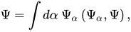
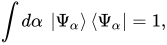
These states are normalized as Permutations work as such; if sSk is a permutation of k objects (for a k-particle state) such that then a nonzero term results. The sign is plus unless s involves an odd number of fermion transpositions, in which case it is minus. The notation is usually abbreviated letting one Greek letter stand for the whole collection describing the state. In abbreviated form the normalization becomes When integrating over free-particle states one writes in this notation where the sum includes only terms such that no two terms are equal modulo a permutation of the particle type indices. The sets of states sought for are supposed to be complete. This is expressed as which could be paraphrased as where for each fixed α, the right hand side is a projection operator onto the state α. Under an inhomogeneous Lorentz transformation (Λ, a), the field transforms according to the rule

where W(Λ, p) is the Wigner rotation and D(j) is the (2j + 1)-dimensional representation of SO(3). By putting Λ = 1, a = (τ, 0, 0, 0), for which U is exp(iHτ), in (1), it immediately follows that so the in and out states sought after are eigenstates of the full Hamiltonian that are necessarily non-interacting due to the absence of mixed particle energy terms. The discussion in the section above suggests that the in states Ψ+ and the out states Ψ should be such that for large positive and negative τ has the appearance of the corresponding package, represented by g, of free-particle states, g assumed smooth and suitably localized in momentum. Wave packages are necessary, else the time evolution will yield only a phase factor indicating free particles, which cannot be the case. The right hand side follows from that the in and out states are eigenstates of the Hamiltonian per above. To formalize this requirement, assume that the full Hamiltonian H can be divided into two terms, a free-particle Hamiltonian H0 and an interaction V, H = H0 + V such that the eigenstates Φγ of H0 have the same appearance as the in- and out-states with respect to normalization and Lorentz transformation properties,


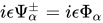
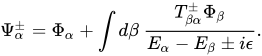
The in and out states are defined as eigenstates of the full Hamiltonian, satisfying for τ → −∞ or τ → +∞ respectively. Define then This last expression will work only using wave packages.From these definitions follow that the in and out states are normalized in the same way as the free-particle states, and the three sets are unitarily equivalent. Now rewrite the eigenvalue equation, where the ± terms has been added to make the operator on the LHS invertible. Since the in and out states reduce to the free-particle states for V → 0, put on the RHS to obtain Then use the completeness of the free-particle states, to finally obtain Here H0 has been replaced by its eigenvalue on the free-particle states. This is the Lippmann–Schwinger equation.


In states expressed as out states

[edit]

The initial states can be expanded in a basis of final states (or vice versa). Using the completeness relation, where |Cm|2 is the probability that the interaction transforms into By the ordinary rules of quantum mechanics, and one may write The expansion coefficients are precisely the S-matrix elements to be defined below.


S-matrix

[edit]

The S-matrix is now defined by[13]

Here α and β are shorthands that represent the particle content but suppresses the individual labels. Associated to the S-matrix there is the S-operator S defined by[13] where the Φγ are free particle states.[13][nb 2] This definition conforms with the direct approach used in the interaction picture. Also, due to unitary equivalence,


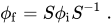
As a physical requirement, S must be a unitary operator. This is a statement of conservation of probability in quantum field theory. But By completeness then, so S is the unitary transformation from in-states to out states. Lorentz invariance is another crucial requirement on the S-matrix.[13][nb 3] The S-operator represents the quantum canonical transformation of the initial in states to the final out states. Moreover, S leaves the vacuum state invariant and transforms in-space fields to out-space fields,[nb 4]

In terms of creation and annihilation operators, this becomes hence A similar expression holds when S operates to the left on an out state. This means that the S-matrix can be expressed as

If S describes an interaction correctly, these properties must be also true:

  • If the system is made up with a single particle in momentum eigenstate |k, then S|k⟩ = |k. This follows from the calculation above as a special case.
  • The S-matrix element may be nonzero only where the output state has the same total momentum as the input state. This follows from the required Lorentz invariance of the S-matrix.

Evolution operator U

[edit]

Define a time-dependent creation and annihilation operator as follows, so, for the fields, where

We allow for a phase difference, given by because for S,

Substituting the explicit expression for U, one has where is the interaction part of the Hamiltonian and is the time ordering.

By inspection, it can be seen that this formula is not explicitly covariant.

Dyson series

[edit]

The most widely used expression for the S-matrix is the Dyson series. This expresses the S-matrix operator as the series: where:

  • denotes time-ordering,
  • denotes the interaction Hamiltonian density which describes the interactions in the theory.

The not-S-matrix

[edit]

Since the transformation of particles from black hole to Hawking radiation could not be described with an S-matrix, Stephen Hawking proposed a "not-S-matrix", for which he used the dollar sign ($), and which therefore was also called "dollar matrix".[14]

See also

[edit]

Remarks

[edit]
  1. ^ This is not true if an open system is studied. Under an influence of an external field the in and out vacua can differ since the external field can produce particles.
  2. ^ Here it is assumed that the full Hamiltonian H can be divided into two terms, a free-particle Hamiltonian H0 and an interaction V, H = H0 + V such that the eigenstates Φγ of H0 have the same appearance as the in- and out-states with respect to normalization and Lorentz transformation properties. See Weinberg (2002), page 110.
  3. ^ If Λ is a (inhomogeneous) proper orthochronous Lorentz transformation, then Wigner's theorem guarantees the existence of a unitary operator U(Λ) acting either on Hi or Hf. A theory is said to be Lorentz invariant if the same U(Λ) acts on Hi and Hf. Using the unitarity of U(Λ), Sβα = ⟨i, β|f, α⟩ = ⟨i, β|U(Λ)U(Λ)|f, α. The right-hand side can be expanded using knowledge about how the non-interacting states transform to obtain an expression, and that expression is to be taken as a definition of what it means for the S-matrix to be Lorentz invariant. See Weinberg (2002), equation 3.3.1 gives an explicit form.
  4. ^ Here the postulate of asymptotic completeness is employed. The in and out states span the same Hilbert space, which is assumed to agree with the Hilbert space of the interacting theory. This is not a trivial postulate. If particles can be permanently combined into bound states, the structure of the Hilbert space changes. See Greiner & Reinhardt 1996, section 9.2.

Notes

[edit]

References

[edit]
Revisions and contributorsEdit on WikipediaRead on Wikipedia
from Grokipedia
The S-matrix, also known as the scattering matrix, is a unitary operator in quantum mechanics and quantum field theory that relates the asymptotic initial states of particles at $ t \to -\infty $ to their asymptotic final states at $ t \to +\infty $, thereby encoding the probabilities and amplitudes for all possible outcomes in scattering processes.[1] It is defined as $ S = \lim_{t_\text{out}, t_\text{in} \to \mp \infty} U(t_\text{out}, t_\text{in}) $, where $ U $ is the time-evolution operator, ensuring that the total probability is conserved through its unitarity property $ S^\dagger S = 1 $.[1] In practice, the S-matrix elements $ \langle f | S | i \rangle $ provide the transition amplitudes from initial state $ |i\rangle $ to final state $ |f\rangle $, often expressed as $ S = 1 + iT $, where $ T $ is the transition matrix related to interaction strengths.[2] The concept of the S-matrix was first introduced by John Archibald Wheeler in 1937 as a tool to describe nuclear reactions using resonating group structures, marking an early attempt to systematize scattering without full wave function solutions.[3] It gained prominence in the 1940s through Werner Heisenberg's development of S-matrix theory, proposed as an alternative framework to quantum field theory for handling high-energy particle interactions, emphasizing observable scattering data over unobservable fields.[4] Heisenberg's approach, detailed in papers from 1943 onward, aimed to resolve divergences in quantum electrodynamics by focusing solely on the S-matrix's analytic properties derived from causality and unitarity.[5] This theory influenced subsequent work, including the bootstrap models of the 1960s and Regge theory, before being largely integrated into standard quantum field theory by the 1970s.[6] Key properties of the S-matrix include its analyticity in the complex energy plane, which stems from causality (effects cannot precede causes) and locality of interactions, leading to dispersion relations that connect real and imaginary parts of amplitudes.[6] Unitarity not only conserves probability but also implies the optical theorem, $ 2 \Im \langle f | T | i \rangle = \sum_n \langle f | T^\dagger | n \rangle \langle n | T | i \rangle $, linking the forward scattering amplitude's imaginary part to total cross-sections.[1] Poincaré invariance ensures the S-matrix commutes with Lorentz transformations, making it a covariant object suitable for relativistic theories.[1] In modern physics, the S-matrix remains central to perturbative calculations in quantum chromodynamics and electroweak theory, as well as non-perturbative approaches like the S-matrix bootstrap, where it serves as the primary observable for constraining effective field theories without relying on underlying Lagrangians.[4] Recent applications extend to amplitude methods in collider experiments and even connections to string theory and chaos in quantum field theory. As of 2024, there has been a resurgence in S-matrix research, highlighted by workshops like the S-Matrix Marathon and advances in the S-matrix bootstrap program.[7][8]

Historical Development

Origins in Early Quantum Mechanics

The concept of the S-matrix emerged from early efforts in quantum mechanics to describe scattering processes without relying on the full solution of the Schrödinger equation, building on foundational ideas about transition probabilities. In 1927, Paul Dirac introduced key precursors through his work on the quantum mechanics of collision processes, where he developed methods to compute scattering amplitudes, laying the groundwork for descriptions of particle transitions.[9] This approach gained practical momentum in nuclear physics with John Archibald Wheeler's 1937 proposal of the S-matrix as a unitary operator mapping initial to final states in scattering reactions. Wheeler formulated the S-matrix within the resonating group structure method to analyze light nuclei and nuclear interactions, allowing predictions of reaction outcomes—such as cross-sections for particle collisions—directly from asymptotic wave functions, bypassing the computationally intensive task of solving the complete many-body Schrödinger equation for complex nuclear systems.[10] Wheeler's non-relativistic framework was significantly extended by Werner Heisenberg during World War II, amid growing frustrations with the infinities plaguing perturbative calculations in quantum field theory (QFT). In papers published in Zeitschrift für Physik from 1943 to 1944, Heisenberg proposed the S-matrix as a fundamental tool for relativistic particle interactions, prioritizing observable scattering amplitudes over unphysical intermediate states and emphasizing principles like causality and unitarity to circumvent renormalization issues.[11] Heisenberg introduced the unitary property as a core postulate, ensuring probability conservation in transitions between free-particle states, which became central to the theory's predictive power for high-energy processes.[11]

Evolution in Quantum Field Theory

In the post-World War II era, the S-matrix formalism underwent significant refinement within relativistic quantum field theory (QFT), particularly through the development of dispersion relations in the 1950s. These relations, derived from causality and unitarity principles, established the analyticity of the S-matrix in the complex energy plane, enabling non-perturbative predictions for scattering amplitudes without relying on underlying field Lagrangians. Pioneering contributions came from Geoffrey Chew and Julian Schwinger, who applied dispersion relations to pion-nucleon scattering, connecting asymptotic behavior at high energies to low-energy experimental data and resolving issues in strong interaction phenomenology.[12][13] A hallmark of this evolution was the bootstrap hypothesis, proposed by Geoffrey Chew in the early 1960s, which posited that the S-matrix could be self-consistently determined solely from its general principles—such as unitarity, crossing symmetry, and analyticity—without invoking elementary particles or fundamental fields. This approach aimed to derive particle masses, widths, and coupling constants as bound states emerging from the S-matrix dynamics itself, offering a democratic view of hadrons as composite excitations. The hypothesis gained traction in strong interaction physics, where it integrated with Regge theory, developed in the late 1950s and 1960s by Tullio Regge and others, to model high-energy scattering via Regge poles and trajectories that interpolated between resonances and particle exchanges. Regge theory successfully described forward scattering peaks and total cross-section behaviors in hadron collisions, providing a framework for extrapolating experimental data beyond perturbative regimes.[14][15][16][17] The S-matrix approach demonstrated early empirical success in interpreting 1950s experiments on pion photoproduction, where dispersion relations predicted multipole amplitudes that matched observations from photon-nucleon interactions at energies up to several hundred MeV, validating the method's non-perturbative power before the dominance of Feynman diagram techniques. By the 1970s, however, the rise of quantum chromodynamics (QCD) as the standard theory of strong interactions—confirmed by asymptotic freedom and deep inelastic scattering data—led to a decline in pure S-matrix methods, as QCD provided a field-theoretic basis for confinement and quark-gluon dynamics. Despite this, S-matrix principles persisted in effective field theories for low-energy phenomena and saw a revival in the 21st century through the AdS/CFT correspondence, where bulk scattering amplitudes in anti-de Sitter space map to boundary conformal field theory correlators, bridging holography and S-matrix analyticity.[18][19][4][20]

Conceptual Foundations

Motivation from Scattering Processes

In scattering processes, particles interact over long distances, transitioning from initial free-particle states to final states that are also asymptotically free, allowing the S-matrix to characterize these interactions without resolving the full dynamics of the collision.[21] This approach arises from the practical difficulties in solving the time-dependent Schrödinger equation for multi-particle systems, where the complexity of entangled wavefunctions and time evolution makes exact solutions infeasible, shifting emphasis to observable transition probabilities between distant asymptotic regimes.[22] As time approaches ±∞, interactions effectively vanish, defining incoming waves from the past and outgoing waves to the future, which the S-matrix maps directly.[21] The elements of the S-matrix, denoted as $ S_{fi} = \langle f | S | i \rangle $, where $ |i\rangle $ and $ |f\rangle $ are initial and final asymptotic states, yield transition probabilities $ |S_{fi}|^2 $ that quantify the likelihood of specific outcomes in scattering experiments.[23] These probabilities underpin the calculation of differential and total cross-sections, essential for predicting reaction rates and comparing theory with experimental data, such as in particle accelerators where cross-sections measure interaction strengths.[24] Historically, the S-matrix concept emerged in nuclear physics to describe collision outcomes in light nuclei without full wavefunction computations, as introduced by John Archibald Wheeler in 1937 for resonating group structures. In quantum field theory, Werner Heisenberg further motivated its development in 1943 to circumvent ultraviolet divergences plaguing perturbative calculations, by parameterizing observables like scattering amplitudes directly through an integral formulation that avoids differential equations and focuses solely on asymptotic behaviors.[5] This strategy ensured finite, unitarity-constrained results for physical processes, preserving probability conservation amid theoretical uncertainties.[25]

General Role and Applications

The S-matrix serves as the fundamental operator in quantum field theory that encodes the probabilities for transitions between free-particle asymptotic states, allowing direct computation of key observables in scattering experiments. Specifically, the differential cross-section for a scattering process is proportional to the square of the magnitude of the relevant S-matrix element, $ \frac{d\sigma}{d\Omega} \propto | \langle f | S | i \rangle |^2 $, where $ |i\rangle $ and $ |f\rangle $ denote the initial and final states, while the total cross-section is obtained by integrating this over all solid angles.[26] These relations enable precise predictions of interaction strengths without relying on intermediate off-shell states. In perturbative quantum field theory, the S-matrix can be expanded using the Dyson series to compute these elements order by order in the coupling constant. Beyond cross-sections, the S-matrix connects to other particle physics observables, including decay rates via the optical theorem, which relates the imaginary part of the forward scattering amplitude to the total cross-section and thus to sum rules over decay channels. Resonances appear as poles in the complex energy plane of the S-matrix, determining their positions and widths, while partial-wave analysis extracts phase shifts that characterize the energy dependence of interactions.[27] These features are crucial for interpreting collider data and modeling unstable particles. The S-matrix finds broad applications across physics disciplines. In nuclear physics, it is used to analyze neutron-proton scattering, where phase shifts derived from S-matrix elements fit experimental data to constrain nucleon-nucleon potentials.[28] In condensed matter physics, the scattering matrix approach describes quantum electron transport in mesoscopic systems, relating transmission probabilities to conductance via Landauer-Büttiker formalism.[29] Analogously, in optics, the S-matrix framework for wave propagation through multilayer structures parallels the Jones matrix, which handles polarization transformations in birefringent media.[30] In axiomatic quantum field theory, the S-matrix is constrained by fundamental postulates: unitarity ensures probability conservation, analyticity arises from causality and locality, and crossing symmetry relates scattering in different channels, providing a non-perturbative foundation independent of Lagrangian details.[6] Modern applications leverage these properties in effective field theories for low-energy quantum chromodynamics (QCD), where S-matrix bootstrap methods bound low-energy constants in chiral perturbation theory to describe pion scattering and nucleon interactions.088) Additionally, S-matrix unitarity imposes bounds on beyond-Standard-Model physics, guiding searches for new particles at the Large Hadron Collider (LHC) by constraining deviations in high-energy scattering amplitudes.

S-matrix in Non-Relativistic Quantum Mechanics

Definition in One Dimension

In one-dimensional non-relativistic quantum mechanics, the S-matrix provides a compact description of particle scattering by a localized potential V(x)V(x), relating the asymptotic forms of the incoming and outgoing wavefunctions. The scattering problem is governed by the time-independent Schrödinger equation,
22md2ψdx2+V(x)ψ(x)=Eψ(x), -\frac{\hbar^2}{2m} \frac{d^2 \psi}{dx^2} + V(x) \psi(x) = E \psi(x),
where E>0E > 0 is the energy of the incident particle, mm is its mass, and \hbar is the reduced Planck's constant. For large x|x|, where V(x)0V(x) \to 0, the solutions reduce to free-particle plane waves with wave number k=2mE/k = \sqrt{2mE}/\hbar. The general asymptotic behavior of the wavefunction ψ(x)\psi(x) is thus
ψ(x)Aeikx+Beikx(x), \psi(x) \sim A e^{ikx} + B e^{-ikx} \quad (x \to -\infty),
ψ(x)Ceikx+Deikx(x+), \psi(x) \sim C e^{ikx} + D e^{-ikx} \quad (x \to +\infty),
where AA and DD represent incoming amplitudes from the left and right, respectively, while BB and CC are outgoing amplitudes to the left and right.[21][31] The S-matrix is defined as the 2×22 \times 2 unitary matrix that maps the incoming amplitudes to the outgoing ones:
(BC)=S(AD), \begin{pmatrix} B \\ C \end{pmatrix} = S \begin{pmatrix} A \\ D \end{pmatrix},
with
S=(rttr). S = \begin{pmatrix} r & t' \\ t & r' \end{pmatrix}.
Here, tt (or tt') is the transmission coefficient, giving the amplitude for the particle to pass through the potential from left to right (or right to left), while rr (or rr') is the reflection coefficient, giving the amplitude for backscattering from left (or right). For time-reversal invariant and real potentials, t=tt = t' and r2+t2=1|r|^2 + |t|^2 = 1, ensuring conservation of probability current.[21][31] The explicit form of SS is obtained by solving the Schrödinger equation numerically or analytically, matching the wavefunction and its derivative at boundaries within the potential region to determine the coefficients.[21]

Unitary Property

In one-dimensional quantum mechanics, the unitarity of the S-matrix arises directly from the conservation of probability, as encoded in the continuity equation derived from the Schrödinger equation. The probability density is ρ(x,t)=ψ(x,t)2\rho(x, t) = |\psi(x, t)|^2, and the continuity equation is ρt+jx=0\frac{\partial \rho}{\partial t} + \frac{\partial j}{\partial x} = 0, where the probability current is j(x,t)=2mi(ψψxψψx)j(x, t) = \frac{\hbar}{2mi} \left( \psi^* \frac{\partial \psi}{\partial x} - \psi \frac{\partial \psi^*}{\partial x} \right).[21] For stationary scattering states of the form ψ(x,t)=ψ(x)eiEt/\psi(x, t) = \psi(x) e^{-iEt/\hbar}, the density ρ\rho is time-independent, implying jx=0\frac{\partial j}{\partial x} = 0 and thus a constant current jj throughout space.[21] Consider a scattering state with incidence from the left, where the asymptotic wave function is ψ(x)eikx+reikx\psi(x) \sim e^{ikx} + r e^{-ikx} as xx \to -\infty and ψ(x)teikx\psi(x) \sim t e^{ikx} as x+x \to +\infty. The current at xx \to -\infty evaluates to j()=km(1r2)j(-\infty) = \frac{\hbar k}{m} (1 - |r|^2), while at x+x \to +\infty it is j(+)=kmt2j(+\infty) = \frac{\hbar k}{m} |t|^2. Equating these constant currents yields t2+r2=1|t|^2 + |r|^2 = 1.[21] A similar relation holds for incidence from the right. The full S-matrix, which linearly relates the outgoing wave amplitudes to the incoming ones as (bLbR)=S(aLaR)\begin{pmatrix} b_L \\ b_R \end{pmatrix} = S \begin{pmatrix} a_L \\ a_R \end{pmatrix} (with aL,aRa_L, a_R incoming and bL,bRb_L, b_R outgoing amplitudes from left and right), takes the form S=(trrt)S = \begin{pmatrix} t & r' \\ r & t' \end{pmatrix}. Unitarity SS=IS^\dagger S = I follows from these flux conservation conditions, ensuring the norms of incoming and outgoing states are preserved.[21] This unitarity has direct implications for elastic scattering: the transmission probability T=t2T = |t|^2 and reflection probability R=r2R = |r|^2 satisfy T+R=1T + R = 1, conserving the total incident probability flux.[21] In one dimension, unitarity also implies the optical theorem, which relates the imaginary part of the forward transmission amplitude Imt(k)\operatorname{Im} t(k) to the total scattering cross-section (analogous to the reflection probability in 1D). Specifically, σtot=2kImf(+)(k,+)\sigma_\text{tot} = \frac{2}{k} \operatorname{Im} f^{(+)}(k, +), where f(+)(k,+)f^{(+)}(k, +) is the forward scattering amplitude related to t(k)t(k).[32] For multi-channel scattering, such as when the particle has internal degrees of freedom (e.g., spin), the S-matrix generalizes to a larger matrix acting on the space of open channels at a given energy; unitarity SS=IS^\dagger S = I holds in this Hilbert space, or block-unitarity for degenerate channel subspaces, again ensuring probability conservation across all accessible channels.[33] Time-reversal symmetry further preserves this unitarity by relating the S-matrix to its transpose in a basis of time-reversed states.[21]

Time-Reversal Symmetry

In one-dimensional non-relativistic quantum mechanics, time-reversal symmetry constrains the S-matrix for scattering processes in systems without magnetic fields or absorption. The time-reversal operator $ T $, an antiunitary operator, acts on a wave function as $ T \psi(x, t) = \psi^*(x, -t) $, where $ * $ denotes complex conjugation, effectively reversing the direction of time while complex-conjugating the state.[34] For a time-independent Hamiltonian $ H $ that commutes with $ T $, satisfying $ T H T^{-1} = H $, this invariance implies that if $ \psi(x, t) $ is a solution to the Schrödinger equation, then $ T \psi(x, t) $ is also a solution.[34] Applying $ T $ to the asymptotic scattering states maps an incident wave from the left (or right) to the time-reversed outgoing wave, leading to specific relations among the S-matrix elements for real-valued, time-independent potentials. In particular, the transmission coefficient is the same from both sides, $ t = t' $. For potentials even under spatial reversal, $ V(-x) = V(x) $, the reflection coefficients satisfy $ r = -r' $, where $ r $ and $ r' $ are the amplitudes for reflection from the left and right, respectively.[35] These relations ensure the symmetry of the S-matrix, $ S(k) = S^T(-k) $, for real-valued potentials.[36] The derivation proceeds by considering the time-reversed scattering solution: under $ T $, the roles of incoming and outgoing waves are interchanged, and for a real potential, the reversed process corresponds to incidence from the opposite direction, yielding the equality of transmission amplitudes and the phase relation between reflections.[35] This symmetry holds as long as the potential is real and time-independent, preserving the invariance $ T H T^{-1} = H $.[36] Time-reversal symmetry is broken by mechanisms such as absorption, introduced via an imaginary component in the potential (e.g., $ V(x) + i W(x) $), or by magnetic fields, which couple through a vector potential odd under $ T $, resulting in non-reciprocal scattering where $ t \neq t' $ and the reflection coefficients become unrelated.[35] In such cases, transmission may differ directionally, and the S-matrix loses its symmetry.[36] In relativistic quantum field theory, these constraints extend through the CPT theorem, which guarantees that any local, Lorentz-invariant theory is invariant under the combined charge conjugation (C), parity (P), and time-reversal (T) transformations, imposing analogous symmetries on the S-matrix elements.[37] Unitarity serves as a complementary constraint, ensuring flux conservation independently of time reversal.[36]

Scattering Coefficients

In one-dimensional quantum mechanics, the scattering coefficients are defined in terms of the elements of the S-matrix, which connects the amplitudes of incoming and outgoing plane waves on either side of the scattering potential. For an incident wave from the left, the asymptotic wave function is expressed as ψ(x)eikx+reikx\psi(x) \to e^{ikx} + r e^{-ikx} for xx \to -\infty and ψ(x)teikx\psi(x) \to t e^{ikx} for x+x \to +\infty, where rr is the reflection amplitude and tt is the transmission amplitude. The transmission coefficient T=t2T = |t|^2 represents the probability that the incident particle is transmitted through the potential, while the reflection coefficient R=r2R = |r|^2 is the probability of reflection.[21] The unitary property of the S-matrix, arising from the conservation of probability current, imposes the constraint T+R=1T + R = 1 for elastic scattering processes. This relation ensures that the incident flux is fully accounted for by transmission and reflection alone, without loss. Experimentally, these coefficients are determined by measuring the ratios of probability currents in the asymptotic regions: the incident current is proportional to 12v|1|^2 v, the reflected to r2v|r|^2 v, and the transmitted to t2v|t|^2 v, where v=k/mv = \hbar k / m is the particle velocity, yielding TT and RR directly from current measurements.[21] The energy dependence of the scattering coefficients is a key feature, with T(E)T(E) varying smoothly or oscillatory for energies above any potential barrier, reflecting interference effects in the scattering process. Near specific energies, T(E)T(E) displays sharp resonant peaks, corresponding to quasi-bound states where the particle is temporarily trapped before transmission or reflection; these resonances manifest as poles of the S-matrix in the complex energy plane just above the real axis. In one dimension, the basis states are plane waves, providing a direct analogy to the partial-wave decomposition in higher dimensions, where the S-matrix is expanded in spherical harmonics and the l=0 (s-wave) component mirrors the 1D plane-wave scattering.[38][21] The optical theorem in one dimension links the imaginary part of the forward scattering amplitude to the total scattering probability (reflection coefficient in 1D), providing an additional consistency check on unitarity.[39]

Optical Theorem in One Dimension

The optical theorem in one dimension is the analog of the relation in higher dimensions that connects the total scattering cross section to the imaginary part of the forward scattering amplitude. In the one-dimensional case, derived from S-matrix theory, the theorem states that the total cross section σ_tot = (2/k) Im f(0), where k is the wave number and f(0) is the forward scattering amplitude in a flux-normalized form. This relation holds for short-range potentials and reflects the conservation of probability flux. The derivation follows directly from the unitarity of the S-matrix, S^\dagger S = I, which ensures the conservation of probability in scattering processes. For an initial state |i\rangle, the unitarity condition implies \sum_f |S_{fi}|^2 = 1, where the sum is over all final states f. In the elastic scattering limit, the forward amplitude corresponds to the diagonal S-matrix element S_{ii}, and the imaginary part arises from the discontinuity across the cut in the complex energy plane. Specifically, 2 Im S_{ii} = \sum_{f \neq i} |S_{fi}|^2, linking the imaginary part of the forward amplitude to the total probability of transition to other states, interpreted as the "cross section" comprising transmission and reflection probabilities. In one dimension, with scattering coefficients t for transmission and r for reflection satisfying |t|^2 + |r|^2 = 1, this yields the flux-normalized form where the imaginary part of the forward amplitude (related to t - 1 in asymptotic wave conventions) equals the total scattering probability normalized by incident flux. A similar flux-normalized expression involves the reflection coefficient as (2/k) Im r(-k) = |t(k)|^2, where r(-k) is the reflection amplitude for incident waves with momentum - \hbar k, connecting the imaginary part to the transmission probability under time-reversal symmetry.[40] This theorem admits an interpretation in terms of shadow scattering or the extinction paradox within one-dimensional waveguides, where the scatterer creates a forward "shadow" due to diffraction, leading to an extinction equal to twice the geometric "size" at high energies—half from actual scattering and half from the diffractive shadow. In 1D quantum or wave propagation, this manifests as the interference between incident and scattered waves reducing the transmitted flux, with the theorem quantifying the extinction via the forward imaginary part.[41] The theorem applies specifically to elastic scattering processes without absorption, where the S-matrix remains unitary due to probability conservation. In cases with absorption or inelastic channels, unitarity is relaxed (||S|| ≤ 1), and the relation generalizes to include absorption in the total extinction, but the pure elastic form requires no loss mechanisms.

Examples in One-Dimensional Potentials

Transfer Matrix Relation

In one-dimensional quantum scattering, the transfer matrix provides an alternative parameterization to the S-matrix by relating the coefficients of the wavefunction on the left and right sides of a scattering potential. Consider the asymptotic form of the wavefunction: to the left of the potential (x → -∞), ψ(x) = A e^{ikx} + B e^{-ikx}, where A is the amplitude of the incoming wave from the left and B is the reflected wave; to the right (x → +∞), ψ(x) = a e^{ikx} + b e^{-ikx}, with a the transmitted wave and b the incoming wave from the right. The transfer matrix M connects these coefficients via
(AB)=M(ab), \begin{pmatrix} A \\ B \end{pmatrix} = M \begin{pmatrix} a \\ b \end{pmatrix},
where M is a 2×2 matrix.[42][43] The unitarity of the S-matrix implies that det M = 1, ensuring conservation of probability current.[43][44] The transfer matrix relates directly to the S-matrix, which typically expresses outgoing amplitudes in terms of incoming ones as \begin{pmatrix} B \ a \end{pmatrix} = S \begin{pmatrix} A \ b \end{pmatrix}. By inverting the transfer matrix relation and adjusting for the direction conventions (swapping incoming and outgoing labels), the S-matrix elements can be expressed in terms of M^{-1}, such as S_{11} = -M_{21}/M_{11} and S_{21} = 1/M_{11} for incidence from the left.[42][44] This connection highlights the equivalence of the two formalisms while emphasizing different aspects of the scattering process. A key advantage of the transfer matrix approach lies in its multiplicative structure for composite systems, such as layered potentials, where the total M is the product of individual transfer matrices for each layer, making it ideal for numerical computations of scattering in complex, piecewise-defined potentials.[43][42] In systems invariant under time reversal, such as those with real-valued potentials, the transfer matrix exhibits symmetry properties M_{11} = M_{22} and M_{12} = -M_{21}, reflecting the reciprocity of transmission and the relation between left and right reflections.[43][44]

Finite Square Well

The finite square well potential serves as a key example for computing the S-matrix in one-dimensional non-relativistic quantum mechanics, particularly illustrating bound states and resonant scattering. Defined as $ V(x) = -V_0 $ for $ |x| < a $ and $ V(x) = 0 $ elsewhere, with $ V_0 > 0 $ and $ a > 0 $, this attractive potential supports a finite number of bound states for $ -V_0 < E < 0 $ and scattering states for $ E > 0 $.[45] For scattering states ($ E > 0 $), the time-independent Schrödinger equation $ -\frac{\hbar^2}{2m} \frac{d^2 \psi}{dx^2} + V(x) \psi = E \psi $ is solved piecewise. In the exterior regions ($ |x| > a $), the wave number is $ k = \sqrt{2mE}/\hbar ,yieldingplanewavesolutions.Insidethewell(, yielding plane wave solutions. Inside the well ( |x| < a $), the effective wave number is $ \kappa = \sqrt{2m(E + V_0)}/\hbar $, also yielding oscillatory solutions. The general wave function for incidence from the left is
ψ(x)={eikx+r(k)eikxx<a,Acos(κx)+Bsin(κx)axa,t(k)eikxx>a, \psi(x) = \begin{cases} e^{ikx} + r(k) e^{-ikx} & x < -a, \\ A \cos(\kappa x) + B \sin(\kappa x) & -a \leq x \leq a, \\ t(k) e^{ikx} & x > a, \end{cases}
where $ r(k) $ and $ t(k) $ are the reflection and transmission amplitudes, respectively.[46] Continuity of $ \psi(x) $ and $ \psi'(x) $ at $ x = \pm a $ provides four equations for the coefficients $ A $, $ B $, $ r(k) $, and $ t(k) $. Solving this system yields the transmission amplitude
t(k)=[cos(2κa)ik2+κ22kκsin(2κa)]1, t(k) = \left[ \cos(2 \kappa a) - i \frac{k^2 + \kappa^2}{2 k \kappa} \sin(2 \kappa a) \right]^{-1},
up to an overall phase factor $ e^{-i 2 k a} $ accounting for the free propagation distance across the well, and the reflection amplitude
r(k)=ik2κ22kκsin(2κa)t(k). r(k) = i \frac{k^2 - \kappa^2}{2 k \kappa} \sin(2 \kappa a) \, t(k).
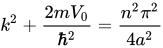
These expressions relate directly to the S-matrix elements for the symmetric potential, with the unitarity condition ensuring $ |t(k)|^2 + |r(k)|^2 = 1 $.[45][46] The transmission probability $ T(k) = |t(k)|^2 $ exhibits perfect transmission ($ T = 1 $, $ R = 0 $) at discrete resonances where $ \sin(2 \kappa a) = 0 $, or $ 2 \kappa a = n \pi $ for integer $ n \geq n_{\min} $, corresponding to energies $ E_n = \frac{n^2 \pi^2 \hbar^2}{8 m a^2} - V_0 > 0 $. These resonances occur at the quasi-bound state energies analogous to those of the infinite square well, manifesting as sharp peaks in $ T(E) $ versus $ E $. For example, with well strength parameter $ z_0 = a \sqrt{2 m V_0}/\hbar \approx 13\pi/4 $, plots of $ T $ versus $ E/V_0 $ show multiple peaks reaching unity, separated by intervals reflecting the well's quantization, with broader low-energy behavior near $ E \approx 0 $.[45] In the limit $ V_0 \to \infty $, the finite well approaches the infinite square well, where transmission vanishes for all $ E > 0 $ as the particle is confined, but for large finite $ V_0 $, $ T(E) $ remains small except at narrow resonant peaks near the infinite well energies $ E_n^{\infty} = \frac{n^2 \pi^2 \hbar^2}{8 m a^2} $, with peak heights of 1 and widths scaling as $ 1/V_0 $. This highlights the role of the finite depth in enabling resonant tunneling without violating unitarity.[46]

Finite Square Barrier

The finite square barrier potential is defined as $ V(x) = V_0 $ for $ |x| < a $ and $ V(x) = 0 $ otherwise, with $ V_0 > 0 $, representing a repulsive scatterer that particles of energy $ E $ may tunnel through if $ E < V_0 $. Inside the barrier region, for $ E < V_0 $, the time-independent Schrödinger equation yields evanescent wave solutions of the form $ e^{\pm \kappa x} $, where $ \kappa = \sqrt{2m(V_0 - E)} / \hbar $ is the decay constant, with $ m $ the particle mass and $ \hbar $ the reduced Planck's constant; these solutions describe the penetration and decay of the wave function without oscillatory propagation.[47][48] The S-matrix elements for this potential, particularly the transmission amplitude $ t(k) $, are obtained by matching the wave functions and their derivatives at the boundaries $ x = \pm a $, where $ k = \sqrt{2mE} / \hbar $ is the wave number outside the barrier. For $ E < V_0 $, the exact transmission coefficient is $ T = |t(k)|^2 = \left[ 1 + \frac{V_0^2 \sinh^2(\kappa \cdot 2a)}{4E(V_0 - E)} \right]^{-1} $, reflecting the probability of tunneling through the full barrier width $ 2a $. At low energies where $ \kappa \cdot 2a \gg 1 $, this approximates to $ T \approx 16 \frac{E}{V_0} \left(1 - \frac{E}{V_0}\right) e^{-2\kappa \cdot 2a} $, demonstrating the exponential suppression of transmission due to the barrier's opacity.[47][48] For $ E > V_0 $, the waves inside the barrier become oscillatory with wave number $ q = \sqrt{2m(E - V_0)} / \hbar $, and the exact transmission amplitude takes the form $ t(k) = \left[ \cos(q \cdot 2a) - i \frac{k^2 + q^2}{2 k q} \sin(q \cdot 2a) \right]^{-1} $, up to an overall phase factor $ e^{-i k \cdot 2a} $ accounting for the free propagation distance across the barrier. This leads to an oscillatory transmission coefficient $ T = |t(k)|^2 = \left[ 1 + \frac{V_0^2 \sin^2(q \cdot 2a)}{4E(E - V_0)} \right]^{-1} $, where $ T $ varies between near-zero and near-unity values depending on the phase $ q \cdot 2a $. Consequently, the reflection coefficient $ R = 1 - T $ approaches 1 at specific energies above the barrier where $ \sin(q \cdot 2a) = \pm 1 $, resulting from destructive interference of the transmitted waves, analogous to the Ramsauer-Townsend effect observed in atomic scattering.[48][49] The unitarity of the S-matrix is preserved in this case, as $ |r(k)|^2 + |t(k)|^2 = 1 $, which aligns with the one-dimensional optical theorem relating the reflection and transmission coefficients.[48]

S-matrix in Relativistic Quantum Field Theory

Interaction Picture

In quantum field theory, the interaction picture serves as a perturbative framework for analyzing scattering processes, enabling the systematic computation of S-matrix elements through time-dependent perturbation theory. This picture, formalized in the unification of earlier approaches by Dyson, separates the dynamics into free evolution and interaction effects, crucial for handling asymptotic behaviors in relativistic theories. The total Hamiltonian is split as $ H = H_0 + V(t) $, where $ H_0 $ is the free-field Hamiltonian governing non-interacting particles, and $ V(t) $ represents the interaction potential, often local in spacetime for relativistic invariance. Free fields under $ H_0 $ obey the Klein-Gordon equation $ (\square + m^2) \phi = 0 $ for scalars or the Dirac equation $ (i \gamma^\mu \partial_\mu - m) \psi = 0 $ for spinors, ensuring canonical quantization and positive-energy solutions.[50] Operators in the interaction picture evolve solely under the free Hamiltonian: $ A_I(t) = e^{i H_0 t} A_S e^{-i H_0 t} $, where $ A_S $ denotes the time-independent Schrödinger-picture operator; this makes interaction-picture fields $ \phi_I(t) $ and $ \psi_I(t) $ satisfy their respective free equations of motion. In contrast, states evolve according to the interaction term: $ i \frac{d}{dt} |\psi(t)\rangle_I = V_I(t) |\psi(t)\rangle_I $, with $ V_I(t) = e^{i H_0 t} V_S(t) e^{-i H_0 t} $. Field operators in the Heisenberg picture, $ A_H(t) = e^{i H t} A_S e^{-i H t} $, incorporate full dynamics but are related to interaction-picture operators via the full evolution operator.[51][50] The solution for state evolution is the time-ordered exponential $ U_I(t, t_0) = T \exp\left( -i \int_{t_0}^t dt' , V_I(t') \right) $, where $ T $ ensures chronological ordering of non-commuting operators at different times, preventing ambiguities in the perturbative expansion. This operator underpins the Dyson series for higher-order corrections, directly leading to S-matrix elements as limits of $ U_I $ from early to late times.[50] The interaction picture thus facilitates the treatment of asymptotic states, where free-particle descriptions hold far from interactions.[51]

Asymptotic In and Out States

In quantum field theory, the asymptotic in-states describe the configuration of free particles approaching from the distant past, corresponding to the limit $ t \to -\infty $ in the interaction picture, where interactions are negligible and particles propagate as solutions to the free-field equations.[52] Similarly, the out-states capture free particles receding to the distant future as $ t \to +\infty $, again behaving as free-particle states in the interaction picture.[1] These states form the basis for defining scattering processes, as the S-matrix connects the in-states to the out-states, encoding the effects of interactions during the intermediate evolution.[52] The in- and out-states are constructed from the respective vacua using creation operators of the free fields. For a single-particle in-state with momentum $ \mathbf{p} $, it is given by $ | \mathbf{p}, \text{in} \rangle = a^\dagger_{\text{in}}(\mathbf{p}) | 0, \text{in} \rangle $, where $ a^\dagger_{\text{in}}(\mathbf{p}) $ is the creation operator for the asymptotic in-field, normalized such that the states have unit norm in the relativistic sense, $ \langle \mathbf{p}, \text{in} | \mathbf{p}', \text{in} \rangle = (2\pi)^3 2 E_{\mathbf{p}} \delta^3(\mathbf{p} - \mathbf{p}') $.[52] Multi-particle in-states are built by applying multiple creation operators to the in-vacuum, for example, for two bosons, $ | \mathbf{p}_1, \mathbf{p}2; \text{in} \rangle = a^\dagger{\text{in}}(\mathbf{p}1) a^\dagger{\text{in}}(\mathbf{p}2) | 0, \text{in} \rangle $, symmetrized appropriately for identical particles.[1] The out-states follow analogously, $ | \mathbf{p}, \text{out} \rangle = a^\dagger{\text{out}}(\mathbf{p}) | 0, \text{out} \rangle $, ensuring the asymptotic vacua $ |0, \text{in}\rangle $ and $ |0, \text{out}\rangle $ coincide in the full theory.[52] In the Heisenberg picture, the full interacting fields $ \phi_H(t, \mathbf{x}) $ approach the free asymptotic fields $ \phi_{\text{as}}(t, \mathbf{x}) $ as $ |t| \to \infty $, reflecting the dilution of interactions over large distances and times.[1] This convergence justifies treating the in- and out-states as eigenstates of the free Hamiltonian $ H_0 = \int \frac{d^3 p}{(2\pi)^3} E_{\mathbf{p}} a^\dagger(\mathbf{p}) a(\mathbf{p}) $, with the full Hamiltonian $ H $ agreeing with $ H_0 $ on the subspace of asymptotic states.[52] The in- and out-states are related through the S-matrix operator via $ | f, \text{out} \rangle = S | i, \text{in} \rangle $, where the unitary nature of $ S $ preserves probabilities, assuming the interactions are adiabatically switched on and off.[1] This connection underpins crossing symmetry, where analytic continuation of S-matrix elements relates scattering processes across different kinematic channels.[52]

Formal Definition of the S-matrix

In relativistic quantum field theory, the S-matrix is formally defined within the interaction picture as the unitary operator that asymptotically maps incoming particle states to outgoing states as interactions switch on and off adiabatically. The explicit expression is
S=limT+,tUI(T,t), S = \lim_{T \to +\infty, \, t \to -\infty} U_I(T, t),
where $ U_I(T, t) $ denotes the time-evolution operator in the interaction picture, given by the time-ordered exponential
UI(T,t)=Texp(itTVI(t)dt). U_I(T, t) = \mathcal{T} \exp\left( -i \int_t^T V_I(t') \, dt' \right).
Here, $ V_I(t) = e^{i H_0 t} V e^{-i H_0 t} $ is the interaction part of the Hamiltonian in the interaction picture, with $ H_0 $ the free Hamiltonian and $ V $ the interaction potential.[53] This limit assumes that interactions vanish sufficiently rapidly at early and late times to allow free-particle asymptotics.[54] The S-matrix acts on asymptotic in-states as $ |f, \text{out} \rangle = S |i, \text{in} \rangle $, connecting the Hilbert space of free incoming particles to that of free outgoing particles.[54] Its unitarity follows directly from the unitarity of the full time-evolution operator, yielding $ S^\dagger S = I $, which preserves probabilities and implies conservation of particle number in the absence of absorption.[53] Locality of interactions further imposes the cluster decomposition property on S, ensuring that distant systems evolve independently.[55] The physical content of the S-matrix resides in its matrix elements $ \langle f, \text{out} | S | i, \text{in} \rangle $, which encode the scattering amplitudes for transitions from initial state $ |i, \text{in} \rangle $ to final state $ |f, \text{out} \rangle $.[53] These amplitudes include a forward-scattering delta function plus interaction contributions. The S-matrix relates to the transition operator (T-matrix) via $ S = I + i T $, where the T-matrix isolates the non-trivial scattering effects; its elements connect to momentum-space amplitudes through the LSZ reduction formula, which extracts on-shell matrix elements from correlation functions without deriving the full procedure here.[53] Causality in quantum field theory implies analytic properties for the S-matrix: it is analytic in the upper half of the complex momentum-squared plane (away from bound-state poles), arising from the time-ordered nature of propagators and the iε prescription that enforces retarded response.

Perturbative Methods

Time Evolution Operator

In the interaction picture of quantum field theory, the time evolution operator $ U(t_2, t_1) $ describes the dynamics of states under the influence of an interaction Hamiltonian $ V_I(t) $, which is the interaction term transformed to evolve with the free Hamiltonian $ H_0 $. This operator is formally defined as the time-ordered exponential
U(t2,t1)=Texp(it1t2VI(t)dt), U(t_2, t_1) = \mathcal{T} \exp\left( -i \int_{t_1}^{t_2} V_I(t) \, dt \right),
where $ \mathcal{T} $ denotes the time-ordering operation, ensuring that operators at later times are placed to the left of those at earlier times in the expansion. This non-perturbative expression, introduced by Freeman Dyson, captures the full time evolution in the interaction picture without assuming weak coupling. The S-matrix, which encodes scattering amplitudes between asymptotic states, is obtained as the limit $ S = U(\infty, -\infty) $, assuming the interaction vanishes at early and late times. Key properties of $ U(t_2, t_1) $ include unitarity, satisfying $ U^\dagger(t_2, t_1) U(t_2, t_1) = 1 $, which follows from the Hermitian nature of the total Hamiltonian and ensures probability conservation in scattering processes, and the initial condition $ U(t, t) = 1 $. Dyson's formulation of time-ordering provides a rigorous way to handle the non-commutativity of operators at different times, enabling consistent perturbative calculations while defining the operator exactly. The interaction picture simplifies the treatment of perturbations by separating the free evolution $ e^{-i H_0 t} $ from the interaction effects, in contrast to the full time evolution operator $ U_\text{full}(t) = e^{-i H t} $, where $ H = H_0 + V $. To justify the asymptotic limits in the S-matrix, the adiabatic theorem is invoked, ensuring that states evolve freely under $ H_0 $ as $ t \to \pm \infty $ when the interaction is switched on and off sufficiently slowly, thus connecting initial and final free-particle states to the interacting dynamics.[56] This framework underpins the identification of in- and out-states as those evolved by $ U $ from the distant past and future, respectively.

Dyson Series Expansion

The Dyson series provides a perturbative expansion for the S-matrix, which is defined as the time-evolution operator $ S = U(\infty, -\infty) $ in the interaction picture of relativistic quantum field theory, where the full Hamiltonian is split into free and interaction parts. This expansion arises from iteratively solving the time-dependent Schrödinger equation in the interaction picture, yielding a power series in the coupling constant of the interaction potential $ V_I(t) $. The series begins with the identity operator and incorporates higher-order corrections through multiple time integrals of the interaction, ensuring proper chronological ordering to handle non-commuting operators at different times.[57] The iterative form of the expansion for the time-evolution operator $ U(t, t_0) $ is given by
U(t,t0)=1+n=1Un(t,t0), U(t, t_0) = 1 + \sum_{n=1}^\infty U_n(t, t_0),
where the first few terms are $ U_1(t, t_0) = -i \int_{t_0}^t dt_1 , V_I(t_1) $ and $ U_2(t, t_0) = (-i)^2 \int_{t_0}^t dt_1 \int_{t_0}^{t_1} dt_2 , T \left[ V_I(t_1) V_I(t_2) \right] $, with $ T $ denoting the time-ordering operator that arranges products of operators in decreasing order of their time arguments. In general, the $ n $-th order term is \begin{equation} U_n(t, t_0) = \frac{(-i)^n}{n!} \int_{t_0}^t dt_1 \cdots \int_{t_0}^t dt_n , T \left[ V_I(t_1) \cdots V_I(t_n) \right], \end{equation} where the factor of $ 1/n! $ accounts for the indistinguishability of the integration variables under time-ordering, and the integrals extend over all times with the $ T $-product enforcing the correct operator sequence. This form was derived by Dyson to systematically compute S-matrix elements order by order in the fine-structure constant.[57] To evaluate matrix elements of these time-ordered products between free-field states, Wick's theorem is applied, which decomposes the $ T $-product into a sum of normal-ordered terms plus all possible full contractions (pairings of field operators) using free-field propagators. In the free-field limit, only fully contracted terms contribute to connected diagrams, facilitating the computation of scattering amplitudes. This theorem, essential for higher-order calculations, reduces the complexity by replacing operator products with c-number contractions. The convergence of the Dyson series is asymptotic rather than absolute, meaning it provides accurate approximations for weak couplings but diverges for strong interactions; nonetheless, it serves as the foundation for renormalization procedures in quantum electrodynamics. Diagrammatically, each term in the series corresponds to Feynman graphs, where vertices represent interactions and lines denote propagators, offering a visual and computational tool for summing infinite sets of diagrams at fixed order.[57] The equivalence between the nested integral form and the time-ordered integral form is proven using Heaviside step functions (theta functions) to express the time-ordering operator explicitly. For the second-order term, for instance,
T[VI(t1)VI(t2)]=θ(t1t2)VI(t1)VI(t2)+θ(t2t1)VI(t2)VI(t1), T \left[ V_I(t_1) V_I(t_2) \right] = \theta(t_1 - t_2) V_I(t_1) V_I(t_2) + \theta(t_2 - t_1) V_I(t_2) V_I(t_1),
and integrating over all $ t_1, t_2 \in [t_0, t] $ yields twice the nested integral $ \int_{t_0}^t dt_1 \int_{t_0}^{t_1} dt_2 V_I(t_1) V_I(t_2) $ (up to the symmetric part if operators commute), with the $ 1/2! $ factor restoring equality; this generalizes to arbitrary $ n $ by summing over all $ n! $ permutations weighted by theta functions.[58]

Relation to Transition Operators

In perturbative quantum field theory, the S-matrix relates asymptotic in- and out-states and is decomposed as $ S = 1 + i T $, where $ T $ is the transition operator (or T-matrix operator) that encodes the non-trivial scattering interactions.[59] The leading-order term in the perturbative expansion of $ T $ is $ T^{(1)} = -i \int_{-\infty}^{\infty} dt , V_I(t) $, with $ V_I(t) $ the interaction Hamiltonian in the interaction picture, and higher-order contributions arise from connected diagrams that capture the irreducible interactions between particles, excluding disconnected vacuum fluctuations.[60] This decomposition ensures that the identity part of $ S $ accounts for no-scattering forward propagation, while $ iT $ isolates the transition amplitudes. The matrix elements of the T-operator are given by $ \langle f | T | i \rangle = i (2\pi)^4 \delta^4(P_f - P_i) M_{fi} $, where $ |i\rangle $ and $ |f\rangle $ are initial and final multi-particle states with total four-momenta $ P_i $ and $ P_f $, respectively, and $ M_{fi} $ is the Lorentz-invariant scattering amplitude.[59] This form arises from the extraction of connected Feynman diagrams in the perturbative expansion, which automatically excludes vacuum bubbles—disconnected loops that do not contribute to physical scattering processes but appear in the full time-evolution operator. The connected structure of $ T $ is enforced by normalizing the S-matrix elements against the vacuum persistence amplitude, ensuring unitarity and causality in the theory.[60] Historically, the T-matrix formalism bridges old-fashioned perturbation theory, which relies on non-covariant time-ordered expansions and energy conservation at each vertex, with modern covariant methods using Feynman diagrams and manifest Lorentz-invariant propagators. In old-fashioned approaches, intermediate states are summed over positive and negative energies without immediate covariance, leading to equivalent results for S-matrix elements but complicating higher-order calculations; covariant perturbation theory, via the Dyson series, generates the T-operator orders more systematically while preserving relativity. In contemporary applications, the T-matrix serves as the irreducible two-particle kernel in the Bethe-Salpeter equation, describing bound-state wave functions as $ \Psi(P, q) = G(q, P) T(P, q) \Psi(P, q) $, where $ G $ is the two-particle propagator and $ T $ sums irreducible interactions beyond ladder approximations.[61]

References

User Avatar
No comments yet.