
Community hub
Recent from talks
Contribute something
Nothing was collected or created yet.
Anemometer
View on Wikipedia

In meteorology, an anemometer (from Ancient Greek άνεμος (ánemos) 'wind' and μέτρον (métron) 'measure') is a device that measures wind speed and direction. It is a common instrument used in weather stations. The earliest known description of an anemometer was by Italian architect and author Leon Battista Alberti (1404–1472) in 1450.
History
[edit]
The anemometer has changed little since its development in the 15th century. Alberti is said to have invented it around 1450. In the ensuing centuries numerous others, including Robert Hooke (1635–1703), developed their own versions, with some mistakenly credited as its inventor. In 1846, Thomas Romney Robinson (1792–1882) improved the design by using four hemispherical cups and mechanical wheels. In 1926, Canadian meteorologist John Patterson (1872–1956) developed a three-cup anemometer, which was improved by Brevoort and Joiner in 1935. In 1991, Derek Weston added the ability to measure wind direction. In 1994, Andreas Pflitsch developed the sonic anemometer.[1]
Velocity anemometers
[edit]Cup anemometers
[edit]
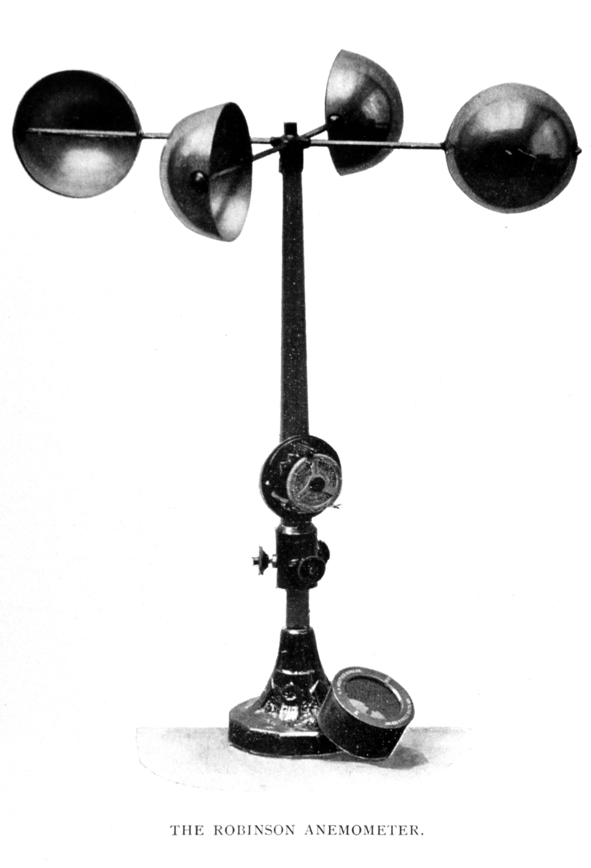
A simple type of anemometer was invented in 1845 by Rev. Dr. John Thomas Romney Robinson of Armagh Observatory. It consisted of four hemispherical cups on horizontal arms mounted on a vertical shaft. The air flow past the cups in any horizontal direction turned the shaft at a rate roughly proportional to the wind's speed. Therefore, counting the shaft's revolutions over a set time interval produced a value proportional to the average wind speed for a wide range of speeds. This type of instrument is also called a rotational anemometer.
Four cup
[edit]With a four-cup anemometer, the wind always has the hollow of one cup presented to it, and is blowing on the back of the opposing cup. Since a hollow hemisphere has a drag coefficient of .38 on the spherical side and 1.42 on the hollow side,[2] more force is generated on the cup that presenting its hollow side to the wind. Because of this asymmetrical force, torque is generated on the anemometer's axis, causing it to spin.
Theoretically, the anemometer's speed of rotation should be proportional to the wind speed because the force produced on an object is proportional to the speed of the gas or fluid flowing past it. However, in practice, other factors influence the rotational speed, including turbulence produced by the apparatus, increasing drag in opposition to the torque produced by the cups and support arms, and friction on the mount point. When Robinson first designed his anemometer, he asserted that the cups moved one-third of the speed of the wind, unaffected by cup size or arm length. This was apparently confirmed by some early independent experiments, but it was incorrect. Instead, the ratio of the speed of the wind and that of the cups, the anemometer factor, depends on the dimensions of the cups and arms, and can have a value between two and a little over three. Once the error was discovered, all previous experiments involving anemometers had to be repeated.
Three cup
[edit]The three-cup anemometer developed by Canadian John Patterson in 1926, and subsequent cup improvements by Brevoort & Joiner of the United States in 1935, led to a cupwheel design with a nearly linear response and an error of less than 3% up to 60 mph (97 km/h). Patterson found that each cup produced maximum torque when it was at 45° to the wind flow. The three-cup anemometer also had a more constant torque and responded more quickly to gusts than the four-cup anemometer.
Three cup wind direction
[edit]The three-cup anemometer was further modified by Australian Dr. Derek Weston in 1991 to also measure wind direction. He added a tag to one cup, causing the cupwheel speed to increase and decrease as the tag moved alternately with and against the wind. Wind direction is calculated from these cyclical changes in speed, while wind speed is determined from the average cupwheel speed.
Three-cup anemometers are currently the industry standard for wind resource assessment studies and practice.
Vane anemometers
[edit]One of the other forms of mechanical velocity anemometer is the vane anemometer. It may be described as a windmill or a propeller anemometer. Unlike the Robinson anemometer, whose axis of rotation is vertical, the vane anemometer must have its axis parallel to the direction of the wind and is therefore horizontal. Furthermore, since the wind varies in direction and the axis has to follow its changes, a wind vane or some other contrivance to fulfill the same purpose must be employed.
A vane anemometer thus combines a propeller and a tail on the same axis to obtain accurate and precise wind speed and direction measurements from the same instrument.[3] The speed of the fan is measured by a revolution counter and converted to a windspeed by an electronic chip. Hence, volumetric flow rate may be calculated if the cross-sectional area is known.
In cases where the direction of the air motion is always the same, as in ventilating shafts of mines and buildings, wind vanes known as air meters are employed, and give satisfactory results.[4]
- Vane anemometers
-
 Vane style of anemometer
 -

-
 Hand-held low-speed vane anemometer
 -
 Hand-held digital anemometer or Byram anenometer.


Hot-wire anemometers
[edit]
Hot wire anemometers use a fine wire (on the order of several micrometres) electrically heated to some temperature above the ambient. Air flowing past the wire cools the wire. As the electrical resistance of most metals is dependent upon the temperature of the metal (tungsten is a popular choice for hot-wires), a relationship can be obtained between the resistance of the wire and the speed of the air.[5] In most cases, they cannot be used to measure the direction of the airflow, unless coupled with a wind vane.
Several ways of implementing this exist, and hot-wire devices can be further classified as CCA (constant current anemometer), CVA (constant voltage anemometer) and CTA (constant-temperature anemometer). The voltage output from these anemometers is thus the result of some sort of circuit within the device trying to maintain the specific variable (current, voltage or temperature) constant, following Ohm's law.
Additionally, PWM (pulse-width modulation) anemometers are also used, wherein the velocity is inferred by the time length of a repeating pulse of current that brings the wire up to a specified resistance and then stops until a threshold "floor" is reached, at which time the pulse is sent again.
Hot-wire anemometers, while extremely delicate, have extremely high frequency-response and fine spatial resolution compared to other measurement methods, and as such are almost universally employed for the detailed study of turbulent flows, or any flow in which rapid velocity fluctuations are of interest.
An industrial version of the fine-wire anemometer is the thermal flow meter, which follows the same concept, but uses two pins or strings to monitor the variation in temperature. The strings contain fine wires, but encasing the wires makes them much more durable and capable of accurately measuring air, gas, and emissions flow in pipes, ducts, and stacks. Industrial applications often contain dirt that will damage the classic hot-wire anemometer.

Laser Doppler anemometers
[edit]In laser Doppler velocimetry, laser Doppler anemometers use a beam of light from a laser that is divided into two beams, with one propagated out of the anemometer. Particulates (or deliberately introduced seed material) flowing along with air molecules near where the beam exits reflect, or backscatter, the light back into a detector, where it is measured relative to the original laser beam. When the particles are in great motion, they produce a Doppler shift for measuring wind speed in the laser light, which is used to calculate the speed of the particles, and therefore the air around the anemometer.[6]

Central spike keeps birds away.
Ultrasonic anemometers
[edit]
Ultrasonic anemometers, first developed in the 1950s, use ultrasonic sound waves to measure wind velocity. They measure wind speed based on the time of flight of sonic pulses between pairs of transducers.[7]
The time that a sonic pulse takes to travel from one transducer to its pair is inversely proportionate to the speed of sound in air plus the wind velocity in the same direction: where is the time of flight, is the distance between transducers, is the speed of sound in air and is the wind velocity. In other words, the faster the wind is blowing, the faster the sound pulse travels. To correct for the speed of sound in air (which varies according to temperature, pressure and humidity) sound pulses are sent in both directions and the wind velocity is calculated using the forward and reverse times of flight: where is the forward time of flight and the reverse.


Because ultrasonic anenometers have no moving parts, they need little maintenance and can be used in harsh environments. They operate over a wide range of wind speeds. They can measure rapid changes in wind speed and direction, taking many measurements each second, and so are useful in measuring turbulent air flow patterns.
Their main disadvantage is the distortion of the air flow by the structure supporting the transducers, which requires a correction based upon wind tunnel measurements to minimize the effect. Rain drops or ice on the transducers can also cause inaccuracies.
Since the speed of sound varies with temperature, and is virtually stable with pressure change, ultrasonic anemometers are also used as thermometers.
Measurements from pairs of transducers can be combined to yield a measurement of velocity in 1-, 2-, or 3-dimensional flow. Two-dimensional (wind speed and wind direction) sonic anemometers are used in applications such as weather stations, ship navigation, aviation, weather buoys and wind turbines. Monitoring wind turbines usually requires a refresh rate of wind speed measurements of 3 Hz,[8] easily achieved by sonic anemometers. Three-dimensional sonic anemometers are widely used to measure gas emissions and ecosystem fluxes using the eddy covariance method when used with fast-response infrared gas analyzers or laser-based analyzers.
Acoustic resonance anemometers
[edit]
Acoustic resonance anemometers are a more recent variant of sonic anemometer. The technology was invented by Savvas Kapartis and patented in 1999.[9] Whereas conventional sonic anemometers rely on time of flight measurement, acoustic resonance sensors use resonating acoustic (ultrasonic) waves within a small purpose-built cavity in order to perform their measurement.

Built into the cavity is an array of ultrasonic transducers, which are used to create the separate standing-wave patterns at ultrasonic frequencies. As wind passes through the cavity, a change in the wave's property occurs (phase shift). By measuring the amount of phase shift in the received signals by each transducer, and then by mathematically processing the data, the sensor is able to provide an accurate horizontal measurement of wind speed and direction.
Because acoustic resonance technology enables measurement within a small cavity, the sensors tend to be typically smaller in size than other ultrasonic sensors. The small size of acoustic resonance anemometers makes them physically strong and easy to heat, and therefore resistant to icing. This combination of features means that they achieve high levels of data availability and are well suited to wind turbine control and to other uses that require small robust sensors such as battlefield meteorology. One issue with this sensor type is measurement accuracy when compared to a calibrated mechanical sensor. For many end uses, this weakness is compensated for by the sensor's longevity and the fact that it does not require recalibration once installed.
Pressure anemometers
[edit]
The first designs of anemometers that measure the pressure were divided into plate and tube classes.
Plate anemometers
[edit]These are the first modern anemometers. They consist of a flat plate suspended from the top so that the wind deflects the plate. In 1450, the Italian art architect Leon Battista Alberti invented the first such mechanical anemometer;[10] in 1663 it was re-invented by Robert Hooke.[11][12] Later versions of this form consisted of a flat plate, either square or circular, which is kept normal to the wind by a wind vane. The pressure of the wind on its face is balanced by a spring. The compression of the spring determines the actual force which the wind is exerting on the plate, and this is either read off on a suitable gauge, or on a recorder. Instruments of this kind do not respond to light winds, are inaccurate for high wind readings, and are slow at responding to variable winds. Plate anemometers have been used to trigger high wind alarms on bridges.
Tube anemometers
[edit]


James Lind's anemometer of 1775 consisted of a vertically mounted glass U tube containing a liquid manometer (pressure gauge), with one end bent out in a horizontal direction to face the wind flow and the other vertical end capped. Though the Lind was not the first, it was the most practical and best known anemometer of this type. If the wind blows into the mouth of a tube, it causes an increase of pressure on one side of the manometer. The wind over the open end of a vertical tube causes little change in pressure on the other side of the manometer. The resulting elevation difference in the two legs of the U tube is an indication of the wind speed. However, an accurate measurement requires that the wind speed be directly into the open end of the tube; small departures from the true direction of the wind causes large variations in the reading.
The successful metal pressure tube anemometer of William Henry Dines in 1892 utilized the same pressure difference between the open mouth of a straight tube facing the wind and a ring of small holes in a vertical tube which is closed at the upper end. Both are mounted at the same height. The pressure differences on which the action depends are very small, and special means are required to register them. The recorder consists of a float in a sealed chamber partially filled with water. The pipe from the straight tube is connected to the top of the sealed chamber and the pipe from the small tubes is directed into the bottom inside the float. Since the pressure difference determines the vertical position of the float this is a measure of the wind speed.[13]
The great advantage of the tube anemometer lies in the fact that the exposed part can be mounted on a high pole, and requires no oiling or attention for years; and the registering part can be placed in any convenient position. Two connecting tubes are required. It might appear at first sight as though one connection would serve, but the differences in pressure on which these instruments depend are so minute, that the pressure of the air in the room where the recording part is placed has to be considered. Thus, if the instrument depends on the pressure or suction effect alone, and this pressure or suction is measured against the air pressure in an ordinary room in which the doors and windows are carefully closed and a newspaper is then burnt up the chimney, an effect may be produced equal to a wind of 10 mi/h (16 km/h); and the opening of a window in rough weather, or the opening of a door, may entirely alter the registration.
While the Dines anemometer had an error of only 1% at 10 mph (16 km/h), it did not respond very well to low winds due to the poor response of the flat plate vane required to turn the head into the wind. In 1918 an aerodynamic vane with eight times the torque of the flat plate overcame this problem.
Pitot tube static anemometers
[edit]Modern tube anemometers use the same principle as in the Dines anemometer, but using a different design. The implementation uses a pitot-static tube, which is a pitot tube with two ports, pitot and static, that is normally used in measuring the airspeed of aircraft. The pitot port measures the dynamic pressure of the open mouth of a tube with pointed head facing the wind, and the static port measures the static pressure from small holes along the side on that tube. The pitot tube is connected to a tail so that it always makes the tube's head face the wind. Additionally, the tube is heated to prevent rime ice formation on the tube.[14] There are two lines from the tube down to the devices to measure the difference in pressure of the two lines. The measurement devices can be manometers, pressure transducers, or analog chart recorders.[15]
Ping-pong ball anemometers
[edit]A common anemometer for basic use is constructed from a ping-pong ball attached to a string. When the wind blows horizontally, it presses on and moves the ball; because ping-pong balls are very lightweight, they move easily in light winds. Measuring the angle between the string-ball apparatus and the vertical gives an estimate of the wind speed.
This type of anemometer is mostly used for middle-school level instruction, which most students make on their own, but a similar device was also flown on the Phoenix Mars Lander.[16]
Effect of density on measurements
[edit]In the tube anemometer the dynamic pressure is actually being measured, although the scale is usually graduated as a velocity scale. If the actual air density differs from the calibration value, due to differing temperature, elevation or barometric pressure, a correction is required to obtain the actual wind speed. Approximately 1.5% (1.6% above 6,000 feet) should be added to the velocity recorded by a tube anemometer for each 1000 ft (5% for each kilometer) above sea-level.
Effect of icing
[edit]At airports, it is essential to have accurate wind data under all conditions, including freezing precipitation. Anemometry is also required in monitoring and controlling the operation of wind turbines, which in cold environments are prone to in-cloud icing. Icing alters the aerodynamics of an anemometer and may entirely block it from operating. Therefore, anemometers used in these applications must be internally heated.[17] Both cup anemometers and sonic anemometers are presently available with heated versions.
Instrument location
[edit]In order for wind speeds to be comparable from location to location, the effect of the terrain needs to be considered, especially in regard to height. Other considerations are the presence of trees, and both natural canyons and artificial canyons (urban buildings). The standard anemometer height in open rural terrain is 10 meters.[18]
See also
[edit]- Air flow meter
- Anemoi, for the ancient origin of the name of this technology
- Anemoscope, ancient device for measuring or predicting wind direction or weather
- Automated airport weather station
- Night of the Big Wind
- Particle image velocimetry
- Savonius wind turbine
- Wind power forecasting
- Wind run
- Windsock, a simple high-visibility indicator of approximate wind speed and direction
Notes
[edit]- ^ "History of the Anemometer". Logic Energy. 2012-06-18.
- ^ Sighard Hoerner's Fluid Dynamic Drag, 1965, pp. 3–17, Figure 32 (pg 60 of 455)
- ^ World Meteorological Organization. "Vane anemometer". Eumetcal. Archived from the original on 8 April 2014. Retrieved 6 April 2014.
- ^ Various (2018-01-01). Encyclopaedia Britannica, 11th Edition, Volume 2, Part 1, Slice 1. Prabhat Prakashan.
- ^ "Hot-wire Anemometer explanation". eFunda. Archived from the original on 10 October 2006. Retrieved 18 September 2006.
- ^ Iten, Paul D. (29 June 1976). "Laser Doppler Anemometer". United States Patent and Trademark Office. Retrieved 18 September 2006.
- ^ Sonic Anemometers (Centre for Atmospheric Science - The University of Manchester), retrieved 29 February 2024
- ^ Giebhardt, Jochen (December 20, 2010). "Chapter 11: Wind turbine condition monitoring systems and techniques". In Dalsgaard Sørensen, John; N Sørensen, Jens (eds.). Wind Energy Systems: Optimising design and construction for safe and reliable operation. Elsevier. pp. 329–349. ISBN 9780857090638.
- ^ Kapartis, Savvas (1999) "Anemometer employing standing wave normal to fluid flow and travelling wave normal to standing wave" U.S. patent 5,877,416
- ^ "Windvanes and anemometers". Scientific itineraries in Tuscany. Museo Galileo - Istituto e Museo di Storia della Scienza.
- ^ Hooke, Robert (1746) [1663]. "A Method for making a History of the Weather". The History of the Royal Society of London. By Sprat, Thomas.
- ^ Walker, Malcolm. "History of the Meteorological Office". Cambridge University Press.
The habit of making weather observations regularly and systematically was encouraged by the Royal Society, and as early as 1663 Hooke presented to the Society his paper titled 'A method for making a history of the weather'
- ^ Dines, W. H. (1892). "Anemometer Comparisons". Quarterly Journal of the Royal Meteorological Society. 18 (83): 168. Bibcode:1892QJRMS..18..165D. doi:10.1002/qj.4970188303. Retrieved 14 July 2014.
- ^ "Instrumentation: Pitot Tube Static Anemometer, Part 1". Mt. Washington Observatory. Archived from the original on 14 July 2014. Retrieved 14 July 2014.
- ^ "Instrumentation: Pitot Tube Static Anemometer, Part 2". Mt. Washington Observatory. Archived from the original on 14 July 2014. Retrieved 14 July 2014.
- ^ "The Telltale project." Archived 20 February 2012 at the Wayback Machine
- ^ Makkonen, Lasse; Lehtonen, Pertti; Helle, Lauri (2001). "Anemometry in Icing Conditions". Journal of Atmospheric and Oceanic Technology. 18 (9): 1457. Bibcode:2001JAtOT..18.1457M. doi:10.1175/1520-0426(2001)018<1457:AIIC>2.0.CO;2.

- ^ Oke, Tim R. (2006). "3.5 Wind speed and direction" (PDF). Initial Guidance to Obtain Representative Meteorological Observations At Urban Sites. Instruments and Observing Methods. Vol. 81. World Meteorological Organization. pp. 19–26. Archived (PDF) from the original on 2022-10-09. Retrieved 4 February 2013.
References
[edit]- Meteorological Instruments, W.E. Knowles Middleton and Athelstan F. Spilhaus, Third Edition revised, University of Toronto Press, Toronto, 1953
- Invention of the Meteorological Instruments, W. E. Knowles Middleton, The Johns Hopkins Press, Baltimore, 1969
External links
[edit]- . Encyclopædia Britannica. Vol. 2 (9th ed.). 1878. pp. 24–26.
- Dines, William Henry (1911). . Encyclopædia Britannica. Vol. 2 (11th ed.). pp. 2–3.
- Description of the development and the construction of an ultrasonic anemometer
- Animation Showing Sonic Principle of Operation (Time of Flight Theory) – Gill Instruments
- Collection of historical anemometer
- Principle of Operation: Acoustic Resonance measurement – FT Technologies
- Thermopedia, "Anemometers (laser doppler)"
- Thermopedia, "Anemometers (pulsed thermal)"
- Thermopedia, "Anemometers (vane)"
- The Rotorvane Anemometer. Measuring both wind speed and direction using a tagged three-cup sensor Archived 2019-09-10 at the Wayback Machine
| International | |
|---|---|
| National | |
| Other | |
Anemometer
View on GrokipediaFundamentals
Definition and Applications
An anemometer is a meteorological instrument designed to measure the speed of wind, and in some cases its direction, by converting the kinetic energy of the moving air or the associated pressure differences into quantifiable electrical or mechanical signals for display or recording.[10] The term "anemometer" originates from the Greek words anemos, meaning "wind," and metron, meaning "measure," reflecting its purpose as a wind-measuring device.[11] Anemometers find essential applications across multiple fields, beginning with meteorology where they are integral to weather stations for real-time monitoring of atmospheric conditions to support forecasting and climate studies.[12] In aviation, they ensure runway safety by assessing crosswinds and gusts that influence aircraft operations during takeoff and landing.[13] For heating, ventilation, and air conditioning (HVAC) systems, anemometers facilitate airflow balancing and duct testing to optimize energy efficiency and indoor air quality.[14] In the wind energy sector, they evaluate potential turbine sites by quantifying wind resources and turbulence patterns to inform placement and performance predictions.[15] Environmental monitoring employs anemometers to track pollutant dispersion and airflow in ecosystems, aiding assessments of air quality and ecological impacts.[16] Additionally, in fluid dynamics research, anemometers contribute to experimental validations of airflow models, such as in computational fluid dynamics studies for vehicle aerodynamics.[17] Over time, anemometers have evolved from early mechanical designs, like cup and vane types reliant on rotating components, to advanced digital sensors, including ultrasonic models that use sound wave propagation for non-contact measurements, enhancing precision and reducing wear.[18] This progression has emphasized reliability in harsh environmental conditions, such as extreme weather or offshore installations, where digital variants with no moving parts withstand corrosion, icing, and high winds better than their mechanical predecessors.[19] Anemometers generally operate through either direct velocity sensing or indirect pressure-based approaches, though specifics vary by design.[10]Core Measurement Principles
Anemometers quantify wind speed through diverse physical principles that convert airflow into measurable signals. Mechanical rotation-based methods, such as those in cup or propeller designs, rely on the torque generated by wind on rotating elements to determine speed from rotational frequency. Thermal dissipation principles, employed in hot-wire anemometers, measure the cooling effect of wind on a heated wire or film, where the rate of heat loss correlates with airflow velocity via King's law relating convective heat transfer to speed. Pressure differential approaches, like those in Pitot-static tubes, exploit Bernoulli's principle to compute speed from the dynamic pressure difference between total and static air pressures. Optical techniques in laser Doppler anemometers detect velocity-induced frequency shifts in scattered laser light from particles in the flow, using the Doppler effect to resolve speed components. Acoustic propagation methods in ultrasonic anemometers assess wind by the transit time of sound pulses between transducers, where wind alters the effective speed of sound along the path.[20][21][8][22][23] A fundamental calibration equation for rotational anemometers expresses indicated wind speed as , where is the indicated speed in meters per second, is the instrument-specific constant (typically in m/s per revolution or Hertz, derived from empirical tunnel testing relating rotation to true speed), and is the rotation frequency in Hertz. This linear relationship assumes steady-state conditions and neglects friction or inertia; derivation involves equating aerodynamic torque to rotational inertia, yielding , simplified empirically where is radius, torque coefficient, moment of inertia, and angular velocity, but practical is obtained via least-squares fit to calibration data. For non-rotational types, analogous relations map output (e.g., voltage in hot-wire or time-of-flight in ultrasonic) to speed through fitted polynomials or physical models.[24][25] Wind speed is reported in standard units including meters per second (m/s) for scientific precision, knots (kt, where 1 m/s ≈ 1.944 kt) for aviation and marine use, and miles per hour (mph, where 1 m/s ≈ 2.237 mph), with conversions facilitating global interoperability. The Beaufort scale provides a qualitative correlation, linking observed effects (e.g., smoke direction at 0–1 Bft, ~0–1 m/s; whole trees in motion at 6 Bft, ~10.8–13.8 m/s) to speed ranges for estimation when instruments fail. While anemometers primarily measure speed as a scalar quantity (magnitude of airflow), full wind velocity as a vector incorporates direction, often via integrated vanes or multi-axis sensors like sonic types that resolve orthogonal components.[26][27][28] Accuracy is influenced by threshold speed, the minimum detectable wind below which response is unreliable due to friction or inertia (typically 0.2–0.5 m/s for modern cup anemometers), and stall speed, the upper limit where aerodynamic stall causes non-linearity or overspeeding (often >40 m/s, beyond linear calibration range). These limits define the operational envelope, with thresholds causing underestimation in light winds and stall leading to errors in gusts; calibration in wind tunnels mitigates but cannot eliminate them.[25][29][30]Historical Development
Early Origins
The earliest conceptual efforts to measure wind can be traced to ancient civilizations, though no surviving devices are known. The Renaissance marked a shift toward more structured mechanical designs. In 1450, Italian architect Leon Battista Alberti invented the first known mechanical anemometer, featuring a swinging plate perpendicular to the wind whose angle of deflection indicated wind force.[31] Advancements continued into the 17th century with empirical refinements. In 1667, English scientist Robert Hooke developed pressure plate anemometers, consisting of a suspended metal plate or hemispherical cup that deflected under wind pressure, allowing for comparative measurements of force intensity.[4] These designs quantified wind effects more systematically than prior iterations, often integrating with barometers for meteorological observations. Early anemometers, however, faced significant limitations: they provided mostly qualitative assessments rather than precise quantitative data, suffered from mechanical vulnerabilities like friction and material wear, and operated without standardized scales, hindering consistent replication across users or locations.[4] Such constraints restricted their utility to basic environmental monitoring until later innovations introduced velocity-focused mechanisms.Major Innovations
In 1775, Scottish physician James Lind introduced a U-shaped tube anemometer, a pressure-based device using a liquid manometer to measure wind pressure differences by the displacement in the tube facing the wind.[32] Around 1850, Swedish admiral Johan Henrik Kreüger developed a pressure plate anemometer for Sweden's first meteorological network, enabling systematic wind force recordings at multiple stations.[7] One of the pivotal advancements in anemometer design occurred in 1846 when Irish physicist John Thomas Romney Robinson introduced the four-cup anemometer, featuring hemispherical cups mounted on horizontal arms attached to a vertical shaft, where the rotational speed of the cups was directly proportional to wind velocity.[31] This innovation marked a shift toward more reliable mechanical measurement by leveraging aerodynamic drag differences between the cups facing into and away from the wind, enabling quantitative wind speed assessments at meteorological stations.[33] In the early 20th century, refinements to cup anemometers addressed limitations in response time and torque variability. Canadian meteorologist John Patterson developed the three-cup anemometer in 1926, reducing the number of cups from four to improve sensitivity and startup at lower wind speeds while maintaining proportional rotation to velocity.[34] This design was further enhanced in 1934 by researchers M. J. Brevoort and U. T. Joyner at the National Advisory Committee for Aeronautics (NACA), who conducted wind tunnel tests on hemispherical and conical cups to minimize aerodynamic torque fluctuations and enhance low-speed performance through optimized cup shapes and arm configurations. The 1920s also saw the practical introduction of hot-wire anemometers, building on the theoretical foundation laid by L. V. King in 1914, who derived equations for convective heat loss from fine wires in fluid flows, allowing velocity inference from cooling rates of electrically heated platinum filaments.[35] These instruments excelled in measuring micro-scale turbulence in aerodynamic research, offering high-frequency response unsuitable for earlier mechanical designs. Mid-20th-century progress introduced non-contact optical and acoustic methods: ultrasonic anemometers emerged in the 1960s, using time-of-flight differences of sound pulses between transducers to compute wind vectors without moving parts, ideal for harsh environments.[36] Similarly, laser Doppler anemometers gained prominence in the 1970s, employing Doppler shifts in laser light scattered by particles in the flow for precise, three-dimensional velocity profiling in laboratory and field settings.[37] Standardization efforts by the World Meteorological Organization (WMO), established in 1950, formalized anemometer protocols in the 1950s, recommending cup anemometer placement at a standard 10-meter height above open terrain to ensure comparable global wind data free from local obstructions.[38] The 1980s and 1990s brought a transition to digital electronics in anemometers, incorporating microprocessors for real-time signal processing, automated calibration, and data logging, which improved accuracy and reduced mechanical wear in operational networks.[39] In the 21st century, anemometer innovations have focused on integration rather than new core types, with post-2000 developments embedding sensors in Internet of Things (IoT) frameworks for remote monitoring in wind farms, enabling predictive maintenance and real-time data transmission to optimize turbine performance.[40] As of November 2025, no fundamentally novel anemometer categories have emerged, but IoT enhancements continue to enhance data reliability in large-scale renewable energy deployments.[40]Velocity Anemometers
Cup Anemometers
Cup anemometers measure wind speed by detecting the rotational speed of hemispherical cups driven by the wind. The standard design consists of three or four lightweight hemispherical or conical cups mounted symmetrically on horizontal arms extending from a central vertical shaft, which rotates freely on low-friction bearings.[41] These cups are typically spaced at equal angles—120 degrees for three-cup models and 90 degrees for four-cup models—to ensure omnidirectional response without dependence on wind direction. Modern constructions often employ lightweight materials such as molded plastic or carbon fiber composites for the cups and arms to minimize inertia and enhance responsiveness.[42] The operation relies on the aerodynamic torque imbalance created by the wind: the concave side of each cup experiences greater drag than the convex side, causing continuous rotation. In steady winds, the rotational frequency is linearly proportional to wind speed, expressed by the equation , where is the wind speed in meters per second, is the rotational frequency in revolutions per second, and is the calibration factor specific to the anemometer, typically ranging from 0.4 to 0.5 m/s per revolution for common models.[43] This factor is determined empirically through calibration in a wind tunnel, accounting for the geometry and the effective drag coefficient ratio between the cup faces, which approximates 2:1 in ideal conditions, leading to the wind speed being roughly half the tangential speed at the cup radius. The full derivation stems from balancing the torque from wind drag on the cups against rotational inertia and friction, resulting in a near-linear response above the starting threshold. In some cup anemometer designs, known as two-wire generator anemometers, the rotating cups drive a small DC or AC generator to produce a voltage proportional to wind speed. The output voltage is constant zero when the anemometer is not spinning (zero wind speed), because no electromotive force is generated without rotation. Key variants include the four-cup design, originally developed by Irish astronomer Thomas Robinson in 1846, which provides higher torque for reliable operation in moderate winds but has a higher starting threshold due to increased mass.[44] In contrast, the three-cup configuration, introduced by Canadian inventor John Patterson in 1926, reduces overall inertia for improved low-speed startup and is now the predominant form in meteorological applications. Some hybrid designs incorporate direction-sensing elements without traditional cups, though these remain less common.[34] Cup anemometers offer robustness for prolonged outdoor exposure, with minimal maintenance needs due to their mechanical simplicity and resistance to environmental factors like dust and moderate precipitation.[41] However, they exhibit a starting threshold of approximately 0.5 m/s, below which rotation ceases, and are prone to overspeeding in turbulent gusts by up to 10-20% due to nonlinear aerodynamic effects at high speeds. The distance constant, a measure of response time, is typically 2-3 meters, meaning the anemometer reaches 63% of its final speed after the wind front travels this distance.[42][45]Vane Anemometers
Vane anemometers integrate wind direction sensing with speed measurement through a mechanical assembly featuring a tail vane and a forward-mounted propeller. The tail vane, typically a lightweight fin, ensures yaw alignment by pivoting the instrument into the prevailing wind, positioning the propeller perpendicular to the airflow for optimal rotation. This design allows the device to capture both vector components of wind in a compact form. Modern iterations employ digital encoders, such as optical or Hall-effect sensors, to convert propeller revolutions into electronic signals for precise data logging and transmission.[46][47][25] During operation, wind imparts torque to the propeller blades once the assembly aligns with the flow, causing rotation at a frequency proportional to the wind velocity. The relationship between wind speed and rotation frequency follows the calibrated equation , where represents the instrument constant derived from empirical testing. Calibration occurs in a wind tunnel, adjusting for variables like blade geometry, bearing friction, and density effects to maintain accuracy, often yielding linear responses over typical ranges with periodic recalibration to account for wear.[48][47][49] Common variants encompass handheld units for HVAC assessments, offering portability and measurement ranges from approximately 0.4 to 30 m/s, and fixed stationary models for meteorological stations that endure prolonged exposure. Three-bladed propellers predominate in these designs, providing aerodynamic efficiency and rotational stability without excessive complexity.[50][51][52] These instruments excel in providing simultaneous wind speed and direction data, enabling vector-resolved profiles essential for site-specific analyses. Drawbacks include delayed response to directional shifts from vane inertia, limiting utility in turbulent conditions, and a starting threshold around 1 m/s, where friction prevents reliable initiation of rotation.[47][53] Vane anemometers entered aviation applications in the mid-20th century for ground-based wind monitoring at airfields, with designs incorporating furling mechanisms—such as hinged tails that feather at excessive speeds—to safeguard against overspeed damage during gusts.[54][55] Vane anemometers are commercially available through online wholesale and retail platforms such as Alibaba and AliExpress. Alibaba offers B2B wholesale options from multiple suppliers, featuring various models including digital variants, with minimum order quantities (MOQ) often ranging from 1 to 100 pieces and prices typically from $10 to $200 per unit depending on specifications, quality, and order volume. AliExpress provides more retail-focused listings but also includes bulk and wholesale deals, with prices generally starting around $15 to $100 and options for purchasing multiple units at discounted rates.[56][57]Hot-Wire Anemometers
Hot-wire anemometers measure fluid velocity through the convective cooling of a fine heated wire exposed to the flow. The sensor typically consists of a thin wire, made of tungsten or platinum-rhodium alloy with a diameter of 5 to 10 μm and length of about 1 mm, stretched taut between two prongs and heated by passing an electric current through it.[58][59] The wire's resistance increases with temperature, enabling precise control and measurement of its thermal state. These devices operate primarily in two modes: constant current anemometry (CCA), where a fixed current is supplied and voltage fluctuations indicate cooling-induced resistance changes, or constant temperature anemometry (CTA), where feedback electronics adjust the current to maintain a constant wire temperature, with the required power serving as the velocity signal.[60][61] CTA is preferred for most applications due to its superior dynamic response to rapid flow fluctuations.[59] The operating principle stems from the increased convective heat transfer from the wire to the surrounding fluid as velocity rises, which cools the wire and necessitates more electrical power to sustain its temperature. This relationship was first theoretically established by L. V. King in 1914, building on earlier thermal convection studies and providing the foundation for hot-wire anemometry. King's derivation begins with the steady-state energy balance for the wire, assuming negligible end conduction losses for sufficiently long wires and ignoring radiation at typical operating temperatures. The electrical power input equals the convective heat loss: where is the current, is the wire resistance at temperature , is the convective heat transfer coefficient, and are the wire diameter and length, and is the fluid temperature.[62] The heat transfer coefficient is nondimensionalized using the Nusselt number , where is the fluid thermal conductivity, leading to King's law: Here, is the Reynolds number based on flow velocity and fluid kinematic viscosity , while , , and are constants determined empirically (King proposed , but Collis and Williams refined it to approximately 0.45 for low Reynolds numbers in air flows).[63] Substituting back, the power or voltage squared in CTA mode follows , where and incorporate wire properties and overheat ratio.[62] Calibration involves exposing the anemometer to a controlled velocity field, such as in a low-speed wind tunnel or calibration jet, and recording the output signal (e.g., voltage in CTA) at multiple known velocities . The data are then fitted to King's law form, often by plotting versus and using nonlinear regression to determine , , and ; this curve is stored for real-time velocity computation during measurements. Calibration must account for fluid properties like temperature and density, as they affect and heat transfer, and is typically repeated periodically due to wire degradation.[64] Variants of hot-wire anemometers include single-wire probes, which measure the velocity magnitude in one-dimensional or aligned flows by sensing total cooling, and crossed-wire arrays (X-wires), where two inclined wires (often at 90 degrees) detect differential cooling to resolve two orthogonal velocity components in two-dimensional flows.[65][66] For three-dimensional velocity vectors, arrays with three or more slanted wires are employed, though they require complex signal processing to disentangle components.[67] Hot-wire anemometers offer high-frequency response exceeding 1 kHz, enabling detailed turbulence measurements, and sensitivity to very low velocities down to 0.05 m/s.[68][69] However, their thin wires are fragile and susceptible to breakage from mechanical shock or vibration, while contamination by dust or particulates alters heat transfer and degrades accuracy, limiting use to clean, indoor environments like wind tunnels rather than outdoor settings. Following King's theoretical work, practical hot-wire anemometers gained prominence in aerodynamic research, particularly for wind tunnel testing starting in the 1940s.[70]Laser Doppler Anemometers
Laser Doppler anemometers (LDAs) are optical instruments that measure fluid velocity by detecting the Doppler shift in light scattered from particles entrained in the flow. The technique relies on the principle that particles moving through a laser beam pattern experience a frequency shift proportional to their velocity component along the measurement direction. Developed in the 1960s, LDAs provide non-intrusive measurements suitable for laboratory and controlled environments, particularly in aerodynamics and fluid dynamics research. The foundational design of an LDA involves splitting a monochromatic laser beam, typically from a helium-neon laser, into two parallel beams using a beam splitter and mirrors. These beams are then focused by lenses to intersect at a small angle within the flow field, creating an interference fringe pattern where alternating bright and dark planes are spaced by , with as the laser wavelength. Tracer particles in the fluid, such as smoke or microspheres, cross these fringes and scatter light toward a photodetector. The scattered light from each beam exhibits a Doppler shift, but due to the differential configuration, the beat frequency detected is the difference, given by , where is the velocity component perpendicular to the fringes. This frequency directly relates to velocity via , enabling precise computation from the measured Doppler frequency.[71] Signal processing in LDAs typically employs a photomultiplier tube or avalanche photodiode to capture the intensity-modulated scattered light, producing a Doppler burst signal. The frequency of this burst is analyzed using fast Fourier transform (FFT) or autocorrelation methods to extract , with validation often based on particle arrival times or pedestal offsets for directionality. Early systems used spectrum analyzers, but modern setups incorporate digital signal processors for real-time validation and bias error correction, ensuring accurate velocity histograms even in turbulent flows. The technique was pioneered by Yeh and Cummins in 1964 using a reference-beam configuration for localized flow measurements. Variants of LDAs include forward-scatter and backward-scatter modes, distinguished by the collection optics position relative to the illumination. Forward-scatter detects light on the opposite side of the flow, offering higher signal-to-noise ratios for low-density seeding but requiring access to both sides of the test section; backward-scatter collects light from the same side, facilitating single-sided measurements in confined spaces like wind tunnels, though with reduced sensitivity. Systems can measure one, two, or three velocity components: 1D setups use a single beam pair for axial velocity, 2D adds an orthogonal pair for transverse components, and 3D employs multiple beam pairs with Bragg cells for frequency shifting to resolve all components without directional ambiguity.[71][72] LDAs offer key advantages, including non-intrusive operation that avoids flow disturbance, high spatial resolution down to micrometers, and excellent temporal resolution for capturing turbulence fluctuations with accuracies typically better than ±0.1% of full scale. They excel in measuring instantaneous velocities over a wide range, from millimeters per second to supersonic speeds, making them ideal for detailed flow diagnostics. However, disadvantages include high cost due to precision optics and lasers, the necessity for seeding the flow with micron-sized particles to ensure sufficient scattering (which may not suit clean or particle-free fluids), and sensitivity to optical misalignment or flow turbidity.[22][73] The technology originated at NASA's Langley Research Center (LaRC) in the mid-1960s, with practical differential Doppler systems developed by Foreman and colleagues in 1966 for gas and liquid flows. By the 1970s, LDAs were widely applied in aerospace research and development, including wind tunnel testing for aircraft and rocket propulsion, enabling precise validation of computational fluid dynamics models.[74]Ultrasonic Anemometers
Ultrasonic anemometers measure wind speed and direction by calculating the time-of-flight differences of ultrasonic sound pulses propagated between pairs of transducers, enabling non-contact detection of wind vectors without mechanical components.[25] The design features pairs of piezoelectric transducers arranged along orthogonal paths, typically separated by path lengths of 10-20 cm, that alternately emit and receive short ultrasonic pulses at frequencies ranging from 40 to 100 kHz. These paths are oriented to capture wind components in horizontal and, for three-dimensional models, vertical directions, allowing simultaneous measurement of speed and direction through vector resolution from multiple axes. In operation, wind alters the effective speed of sound propagation: the pulse travels faster downstream and slower upstream relative to the wind direction, producing measurable time differences. The wind speed component along a path is derived from the equation where is the fixed path length, and are the upstream and downstream transit times, and is the angle between the wind vector and the path axis; sound speed is accounted for via the average transit time to correct for temperature and humidity effects.[75][76] Variants include two-dimensional (2D) configurations with transducers aligned for horizontal wind components and three-dimensional (3D) setups using additional orthogonal paths for full vector measurement, including vertical velocity crucial for turbulence studies. An acoustic resonance subtype employs continuous standing waves between transducers instead of pulsed transmission, enhancing sensitivity to low wind speeds and reducing power requirements through phase-shift detection rather than time-of-flight. Ultrasonic anemometers were first commercialized in the 1970s for meteorological research, with the acoustic resonance variant patented in the late 1990s to enable low-power, compact deployments in remote or battery-operated systems.[77][78] Key advantages include the absence of moving parts, which eliminates friction and wear, and a rapid response frequency of 10-50 Hz, permitting accurate capture of turbulent fluctuations and gusts in atmospheric boundary layer studies. They also provide inherent virtual temperature measurements from sound speed variations. However, performance degrades in heavy rain or fog due to acoustic signal attenuation by water droplets, and their higher manufacturing complexity results in elevated costs compared to traditional mechanical sensors.[25][79]Pressure Anemometers
Plate Anemometers
Plate anemometers measure wind speed by quantifying the drag force or deflection produced by wind acting on a flat or curved surface, such as a plate, hemisphere, or sphere. The design typically involves a lightweight plate or similar element suspended on a spring, pivot, or thread, allowing it to swing or compress in response to wind pressure. The angle of deflection or the restoring force required to maintain equilibrium is then measured to infer wind velocity. This approach relies on the principle that dynamic wind pressure increases with the square of the speed, providing a direct mechanical indication without complex electronics.[4] The operation of a plate anemometer is governed by the aerodynamic drag force equation, , where is the drag force, is the drag coefficient (typically around 1.2 for a flat plate perpendicular to the flow), is air density, is the projected area of the plate, and is wind speed. This force causes the plate to deflect until balanced by a restoring mechanism, such as spring tension, with the deflection angle proportional to under steady conditions. A vane often orients the plate into the wind for accurate perpendicular exposure. Air density influences the measurement, though corrections can account for variations.[4][80] Early variants include the swinging-plate design invented by Leon Battista Alberti in 1450, featuring a disc suspended from a rotating axis that tilts under wind pressure. Another variant, the pressure plate anemometer refined by Johan Henrik Kreüger around 1850, employed a flat plate with a vane for directional alignment and was integrated into early meteorological networks. The ping-pong ball anemometer, a portable educational adaptation using a lightweight sphere suspended by a thread, measures deflection with a protractor and has been popular in science education since the mid-20th century. These were widely used in early meteorology for their straightforward construction.[4][7][81] Plate anemometers offer advantages in simplicity and low cost, requiring minimal materials and no power source, making them suitable for basic field or educational applications. However, their response is inherently nonlinear due to the quadratic dependence on velocity, complicating calibration for precise measurements, and they are sensitive to turbulence, which can cause erratic deflections and reduce accuracy in unsteady flows.[80][82]Tube Anemometers
Tube anemometers, particularly the Pitot-static type, measure fluid velocity by detecting the difference between total and static pressures within a flowing medium.[83] The device consists of a forward-facing Pitot tube that captures total pressure, which includes both static and dynamic components, and separate static ports that sense ambient static pressure perpendicular to the flow.[83] This pressure differential, denoted as Δp, is typically measured using a manometer for low-speed applications or a pressure transducer for higher-precision or dynamic environments.[84] The operation relies on Bernoulli's principle, which relates pressure, velocity, and density in fluid flow. For incompressible flows, the velocity v is calculated aswhere ρ is the fluid density.[83] In compressible flows, such as those encountered in high-speed aviation, corrections account for density variations and temperature effects using isentropic flow relations. The Mach number M is derived from the total-to-static pressure ratio:
where p_o is total pressure, p is static pressure, and γ is the specific heat ratio (approximately 1.4 for air); velocity is then v = M √(γ R T), with R the gas constant and T the static temperature. For supersonic flows, additional shock wave corrections apply via the Rayleigh Pitot formula to adjust for the bow shock ahead of the tube. The Pitot tube was invented in 1732 by French engineer Henri Pitot to measure water velocity in rivers, marking an early application of pressure-based flow sensing.[85] The addition of static pressure ports to form the modern Pitot-static configuration evolved in the 19th and early 20th centuries, enabling accurate airspeed determination.[85] Pitot-static tubes became a standard in aviation by the 1920s, integrated into aircraft instruments for airspeed and altitude measurement. Variants include the full Pitot-static probe used in aircraft, where static pressure also informs altimeters and vertical speed indicators, providing comprehensive flight data.[86] Simpler Pitot tubes, without dedicated static ports, are employed in ductwork for industrial airflow monitoring, relying on separate static pressure references.[87] These anemometers offer high accuracy, typically within ±1% of true velocity when properly calibrated, and robust construction suitable for harsh environments.[88] However, they require precise knowledge of fluid density for velocity computation, which varies with temperature and altitude, and are prone to clogging from debris or ice, potentially leading to erroneous readings.[89][90]