Recent from talks
Nothing was collected or created yet.
Bivariate analysis
View on Wikipedia
Bivariate analysis is one of the simplest forms of quantitative (statistical) analysis.[1] It involves the analysis of two variables (often denoted as X, Y), for the purpose of determining the empirical relationship between them.[1]
Bivariate analysis can be helpful in testing simple hypotheses of association. Bivariate analysis can help determine to what extent it becomes easier to know and predict a value for one variable (possibly a dependent variable) if we know the value of the other variable (possibly the independent variable) (see also correlation and simple linear regression).[2]
Bivariate analysis can be contrasted with univariate analysis in which only one variable is analysed.[1] Like univariate analysis, bivariate analysis can be descriptive or inferential. It is the analysis of the relationship between the two variables.[1] Bivariate analysis is a simple (two variable) special case of multivariate analysis (where multiple relations between multiple variables are examined simultaneously).[1]
Bivariate Regression
[edit]
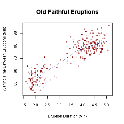
Regression is a statistical technique used to help investigate how variation in one or more variables predicts or explains variation in another variable. Bivariate regression aims to identify the equation representing the optimal line that defines the relationship between two variables based on a particular data set. This equation is subsequently applied to anticipate values of the dependent variable not present in the initial dataset. Through regression analysis, one can derive the equation for the curve or straight line and obtain the correlation coefficient.
Simple Linear Regression
[edit]Simple linear regression is a statistical method used to model the linear relationship between an independent variable and a dependent variable. It assumes a linear relationship between the variables and is sensitive to outliers. The best-fitting linear equation is often represented as a straight line to minimize the difference between the predicted values from the equation and the actual observed values of the dependent variable.

Equation:
: independent variable (predictor)
: dependent variable (outcome)
: slope of the line
: -intercept
Least Squares Regression Line (LSRL)
[edit]The least squares regression line is a method in simple linear regression for modeling the linear relationship between two variables, and it serves as a tool for making predictions based on new values of the independent variable. The calculation is based on the method of the least squares criterion. The goal is to minimize the sum of the squared vertical distances (residuals) between the observed y-values and the corresponding predicted y-values of each data point.
Bivariate Correlation
[edit]A bivariate correlation is a measure of whether and how two variables covary linearly, that is, whether the variance of one changes in a linear fashion as the variance of the other changes.
Covariance can be difficult to interpret across studies because it depends on the scale or level of measurement used. For this reason, covariance is standardized by dividing by the product of the standard deviations of the two variables to produce the Pearson product–moment correlation coefficient (also referred to as the Pearson correlation coefficient or correlation coefficient), which is usually denoted by the letter “r.”[3]
Pearson's correlation coefficient is used when both variables are measured on an interval or ratio scale. Other correlation coefficients or analyses are used when variables are not interval or ratio, or when they are not normally distributed. Examples are Spearman's correlation coefficient, Kendall's tau, Biserial correlation, and Chi-square analysis.

Three important notes should be highlighted with regard to correlation:
- The presence of outliers can severely bias the correlation coefficient.
- Large sample sizes can result in statistically significant correlations that may have little or no practical significance.
- It is not possible to draw conclusions about causality based on correlation analyses alone.
When there is a dependent variable
[edit]If the dependent variable—the one whose value is determined to some extent by the other, independent variable— is a categorical variable, such as the preferred brand of cereal, then probit or logit regression (or multinomial probit or multinomial logit) can be used. If both variables are ordinal, meaning they are ranked in a sequence as first, second, etc., then a rank correlation coefficient can be computed. If just the dependent variable is ordinal, ordered probit or ordered logit can be used. If the dependent variable is continuous—either interval level or ratio level, such as a temperature scale or an income scale—then simple regression can be used.
If both variables are time series, a particular type of causality known as Granger causality can be tested for, and vector autoregression can be performed to examine the intertemporal linkages between the variables.
When there is not a dependent variable
[edit]When neither variable can be regarded as dependent on the other, regression is not appropriate but some form of correlation analysis may be.[4]
Graphical methods
[edit]Graphs that are appropriate for bivariate analysis depend on the type of variable. For two continuous variables, a scatterplot is a common graph. When one variable is categorical and the other continuous, a box plot is common and when both are categorical a mosaic plot is common. These graphs are part of descriptive statistics.
See also
[edit]References
[edit]- ^ a b c d e Earl R. Babbie, The Practice of Social Research, 12th edition, Wadsworth Publishing, 2009, ISBN 0-495-59841-0, pp. 436–440
- ^ Bivariate Analysis, Sociology Index
- ^ Sandilands, Debra (Dallie) (2014). "Bivariate Analysis". Encyclopedia of Quality of Life and Well-Being Research. Springer. pp. 416–418. doi:10.1007/978-94-007-0753-5_222. ISBN 978-94-007-0753-5.
- ^ Chatterjee, Samprit (2012). Regression analysis by example. Hoboken, New Jersey: Wiley. ISBN 978-0470905845.
Bivariate analysis
View on GrokipediaFundamentals
Definition and Scope
Bivariate analysis encompasses statistical methods designed to examine and describe the relationships between exactly two variables, assessing aspects such as the strength, direction, and form of their association.[4] This approach focuses on bivariate data, where one variable is often treated as independent (explanatory) and the other as dependent (outcome), enabling researchers to explore potential patterns without assuming causality.[5] The scope of bivariate analysis extends to various data types, including continuous, discrete, and categorical variables, making it versatile for applications across fields like social sciences, medicine, and economics.[3] It stands in contrast to univariate analysis, which involves a single variable to describe its distribution or central tendencies, and multivariate analysis, which handles interactions among three or more variables for more complex modeling.[6] Historically, bivariate analysis originated in 19th-century statistics, with Francis Galton introducing key concepts like regression to the mean through studies on heredity in the 1880s, and Karl Pearson formalizing correlation measures around 1896 to quantify variable relationships.[7] The primary purpose of bivariate analysis is to identify underlying patterns in data, test hypotheses regarding variable associations, and provide foundational insights that can inform subsequent predictive modeling, such as simple regression techniques.[3] By evaluating whether observed relationships are statistically significant or attributable to chance, it supports evidence-based conclusions while emphasizing that correlation does not imply causation.[4] Graphical tools, like scatterplots, often complement these methods to visualize associations visually.[6]Types of Variables Involved
In bivariate analysis, variables are classified based on their measurement scales, which determine the appropriate analytical approaches. Quantitative variables include continuous types, which can take any value within a range, such as height in meters or temperature in Celsius (interval scale, where differences are meaningful but ratios are not due to the arbitrary zero point), and ratio scales like weight in kilograms, which have a true zero and allow for meaningful ratios.[8][9] Discrete variables, a subset of quantitative data, consist of countable integers, such as the number of children in a family or daily phone calls received.[10][8] Qualitative variables are categorical, divided into nominal, which lack inherent order (e.g., eye color or gender), and ordinal, which have a ranked order but unequal intervals (e.g., education levels from elementary to postgraduate or Likert scale responses from "strongly disagree" to "strongly agree").[8][10][9] The pairings of these variable types shape bivariate analysis strategies. Continuous-continuous pairings, like temperature and ice cream sales, enable examination of linear relationships using methods such as correlation.[8][11] Continuous-categorical pairings, such as income (continuous) and gender (nominal), often involve group comparisons like t-tests for two categories or ANOVA for multiple.[11][10] Categorical-categorical pairings, for instance, smoking status (nominal) and disease presence (nominal) or voting preference (ordinal) and age group (ordinal), rely on contingency tables to assess associations.[8][11] These classifications carry key implications for method selection: continuous variable pairs generally suit parametric techniques assuming normality and equal variances, while categorical pairs necessitate non-parametric approaches or contingency table methods to handle unordered or ranked data without assuming underlying distributions.[8][12] For example, Pearson correlation fits continuous pairs like height and weight, whereas chi-square tests apply to categorical pairs like gender and voting preference.[11][12]Measures of Linear Association
Covariance
Covariance is a statistical measure that quantifies the extent to which two random variables vary together, capturing the direction and degree of their linear relationship. A positive covariance indicates that the variables tend to increase or decrease in tandem, a negative value signifies that one tends to increase as the other decreases, and a value of zero suggests no linear dependence between them.[13] This measure serves as a foundational building block for understanding bivariate associations, though it does not imply causation.[14] The sample covariance between two variables and , based on observations, is given by the formula where and denote the sample means of and , respectively.[15] This estimator is unbiased for the population covariance and uses the divisor to account for degrees of freedom in the sample.[16] The sign of the covariance reflects the direction of co-variation, but its magnitude is sensitive to the units and scales of the variables involved.[14] In terms of interpretation, the units of covariance are the product of the units of the two variables—for example, if one variable is measured in inches and the other in pounds, the covariance would be in inch-pounds—making direct comparisons across different datasets challenging without normalization.[17] Consider a sample of adult heights (in inches) and weights (in pounds): taller individuals often weigh more, yielding a positive covariance value, illustrating how greater-than-average height deviations align with greater-than-average weight deviations.[18] Despite its utility, covariance has notable limitations: it lacks a standardized range (unlike measures bounded between -1 and 1), so values cannot be directly interpreted in terms of strength without considering variable scales, and it is not comparable across studies with differing units or variances.[14] Additionally, while the sign indicates direction, the absolute value does not provide a scale-invariant assessment of association strength.[13]Pearson Correlation Coefficient
The Pearson correlation coefficient, also known as the Pearson product-moment correlation coefficient, is a standardized measure of the strength and direction of the linear relationship between two continuous variables, ranging from -1 to +1, where -1 indicates a perfect negative linear association, +1 a perfect positive linear association, and 0 no linear association.[19][20] It was developed by Karl Pearson as an extension of earlier work on regression and inheritance, providing a scale-invariant alternative to covariance by normalizing the latter with the standard deviations of the variables.[19] The formula for the sample Pearson correlation coefficient is given by: where and are the sample means of variables and , is the sample covariance, and and are the sample standard deviations.[20] To calculate , first compute the means and ; then determine the deviations and for each paired observation; next, sum the products of these deviations to obtain the numerator (covariance term) and sum the squared deviations separately for the denominator components; finally, divide the covariance by the product of the standard deviations.[20] Interpretation focuses on the value of : the absolute value indicates the strength of the linear association, with values near 0 suggesting weak or no linear relationship and values near 1 suggesting strong linear relationship, while the sign denotes direction (positive for direct, negative for inverse). For example, a strong positive correlation (r close to 1) between variables like study time and exam performance would indicate that higher values of one tend to associate with higher values of the other. To assess statistical significance, a t-test is used under the null hypothesis of no population correlation (): with degrees of freedom , where is the sample size; the resulting t-value is compared to a t-distribution to obtain a p-value.[21] The method assumes linearity in the relationship between variables, interval or ratio level data, and bivariate normality (i.e., each variable is normally distributed and their joint distribution is normal), with brief consideration for homoscedasticity in related inference, though violations may affect significance testing more than the coefficient itself.[22][20]Non-Parametric and Categorical Measures
Spearman Rank Correlation
The Spearman rank correlation coefficient, denoted as , is a nonparametric measure of the strength and direction of the monotonic association between two variables, assessing how well the relationship can be described by a monotonically increasing or decreasing function rather than assuming linearity.[23] Introduced by Charles Spearman in 1904, it operates by converting the original data into ranks, making it suitable for detecting associations where the raw data may not meet parametric assumptions.[23] The coefficient ranges from -1, indicating a perfect negative monotonic relationship where higher ranks in one variable correspond to lower ranks in the other, to +1, indicating a perfect positive monotonic relationship, with 0 signifying no monotonic association.[24] The formula for the Spearman rank correlation coefficient is given by where represents the difference between the ranks of the -th paired observations from the two variables, and is the number of observations.[23] To calculate , the values of each variable are first converted to ranks, typically assigning rank 1 to the smallest value and rank to the largest, with the process performed separately for each variable.[25] The rank differences are then computed for each pair, squared, and summed before substitution into the formula.[26] In cases of tied values within a variable, the average of the tied ranks is assigned to each tied observation to maintain consistency—for example, if two values tie for second and third place, both receive a rank of 2.5.[25] The interpretation of is analogous to that of the Pearson correlation coefficient in terms of strength and direction but focuses on monotonic rather than strictly linear relationships, offering greater robustness to outliers and departures from normality since it relies on ranks rather than raw scores.[24] Statistical significance of can be assessed through permutation tests, which reshuffle the paired ranks to generate an empirical null distribution, or by comparing the observed value to critical values from standard statistical tables.[27] Spearman rank correlation is recommended for analyzing non-normally distributed continuous data, ordinal variables, or situations where a nonlinear but monotonic relationship is anticipated, as these conditions violate the assumptions of parametric alternatives like Pearson's method.[24] For example, in socioeconomic research, a between ranked levels of education (e.g., high school, bachelor's, graduate) and income brackets might indicate a strong positive monotonic trend, where higher education consistently associates with higher income without assuming a straight-line relationship.[24]Chi-Square Test of Independence
The chi-square test of independence is a non-parametric statistical test used to assess whether there is a significant association between two categorical variables in a bivariate analysis. It evaluates the null hypothesis that the variables are independent, implying no relationship between their distributions, against the alternative hypothesis that they are dependent. This test is particularly suited for nominal data organized in contingency tables, where it compares observed frequencies to those expected under independence.[28] The test statistic is computed using the formula where represents the observed frequency in the -th row and -th column of the contingency table, and is the expected frequency for that cell, calculated as , with the sums denoting row and column marginal totals and the grand total, respectively. Under the null hypothesis, this statistic approximately follows a chi-square distribution with degrees of freedom , where and are the number of rows and columns.[29] To perform the test, the following steps are followed:- Construct a contingency table displaying the observed frequencies for the cross-classification of the two categorical variables, ensuring the data represent a random sample.
- Calculate the expected frequencies for each cell using the marginal totals and grand total as specified in the formula.
- Compute the chi-square statistic by summing the squared differences between observed and expected frequencies, each divided by the expected frequency.
- Determine the degrees of freedom and obtain the p-value from the chi-square distribution (typically using statistical software or tables for the right-tailed test).
- Compare the p-value to a significance level (e.g., ); if the p-value is less than , reject the null hypothesis of independence.[30]
| Republican | Democrat | Independent | Total | |
|---|---|---|---|---|
| Male | 200 | 150 | 50 | 400 |
| Female | 250 | 300 | 50 | 600 |
| Total | 450 | 450 | 100 | 1,000 |
