Recent from talks
Nothing was collected or created yet.
One- and two-tailed tests
View on Wikipedia

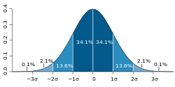
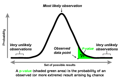
In statistical significance testing, a one-tailed test and a two-tailed test are alternative ways of computing the statistical significance of a parameter inferred from a data set, in terms of a test statistic. A two-tailed test is appropriate if the estimated value is greater or less than a certain range of values, for example, whether a test taker may score above or below a specific range of scores. This method is used for null hypothesis testing and if the estimated value exists in the critical areas, the alternative hypothesis is accepted over the null hypothesis. A one-tailed test is appropriate if the estimated value may depart from the reference value in only one direction, left or right, but not both.[1] An example can be whether a machine produces more than one-percent defective products. In this situation, if the estimated value exists in one of the one-sided critical areas, depending on the direction of interest (greater than or less than), the alternative hypothesis is accepted over the null hypothesis. Alternative names are one-sided and two-sided tests; the terminology "tail" is used because the extreme portions of distributions, where observations lead to rejection of the null hypothesis, are small and often "tail off" toward zero as in the normal distribution, colored in yellow, or "bell curve", pictured on the right and colored in green.
Applications
[edit]One-tailed tests are used for asymmetric distributions that have a single tail, such as the chi-squared distribution, which are common in measuring goodness-of-fit, or for one side of a distribution that has two tails, such as the normal distribution, which is common in estimating location; this corresponds to specifying a direction. Two-tailed tests are only applicable when there are two tails, such as in the normal distribution, and correspond to considering either direction significant.[2][3]
In the approach of Ronald Fisher, the null hypothesis H0 will be rejected when the p-value of the test statistic is sufficiently extreme (vis-a-vis the test statistic's sampling distribution) and thus judged unlikely to be the result of chance. This is usually done by comparing the resulting p-value with the specified significance level, denoted by , when computing the statistical significance of a parameter. In a one-tailed test, "extreme" is decided beforehand as either meaning "sufficiently small" or meaning "sufficiently large" – values in the other direction are considered not significant. One may report that the left or right tail probability as the one-tailed p-value, which ultimately corresponds to the direction in which the test statistic deviates from H0.[4] In a two-tailed test, "extreme" means "either sufficiently small or sufficiently large", and values in either direction are considered significant.[5] For a given test statistic, there is a single two-tailed test, and two one-tailed tests, one each for either direction. When provided a significance level , the critical regions would exist on the two tail ends of the distribution with an area of each for a two-tailed test. Alternatively, the critical region would solely exist on the single tail end with an area of for a one-tailed test. For a given significance level in a two-tailed test for a test statistic, the corresponding one-tailed tests for the same test statistic will be considered either twice as significant (half the p-value) if the data is in the direction specified by the test, or not significant at all (p-value above ) if the data is in the direction opposite of the critical region specified by the test.
For example, if flipping a coin, testing whether it is biased towards heads is a one-tailed test, and getting data of "all heads" would be seen as highly significant, while getting data of "all tails" would be not significant at all (p = 1). By contrast, testing whether it is biased in either direction is a two-tailed test, and either "all heads" or "all tails" would both be seen as highly significant data. In medical testing, while one is generally interested in whether a treatment results in outcomes that are better than chance, thus suggesting a one-tailed test; a worse outcome is also interesting for the scientific field, therefore one should use a two-tailed test that corresponds instead to testing whether the treatment results in outcomes that are different from chance, either better or worse.[6] In the archetypal lady tasting tea experiment, Fisher tested whether the lady in question was better than chance at distinguishing two types of tea preparation, not whether her ability was different from chance, and thus he used a one-tailed test.
Coin flipping example
[edit]In coin flipping, the null hypothesis is a sequence of Bernoulli trials with probability 0.5, yielding a random variable X which is 1 for heads and 0 for tails, and a common test statistic is the sample mean (of the number of heads) If testing for whether the coin is biased towards heads, a one-tailed test would be used – only large numbers of heads would be significant. In that case a data set of five heads (HHHHH), with sample mean of 1, has a chance of occurring, (5 consecutive flips with 2 outcomes - ((1/2)^5 =1/32). This would have and would be significant (rejecting the null hypothesis) if the test was analyzed at a significance level of (the significance level corresponding to the cutoff bound). However, if testing for whether the coin is biased towards heads or tails, a two-tailed test would be used, and a data set of five heads (sample mean 1) is as extreme as a data set of five tails (sample mean 0). As a result, the p-value would be and this would not be significant (not rejecting the null hypothesis) if the test was analyzed at a significance level of .
History
[edit]
The p-value was introduced by Karl Pearson[7] in the Pearson's chi-squared test, where he defined P (original notation) as the probability that the statistic would be at or above a given level. This is a one-tailed definition, and the chi-squared distribution is asymmetric, only assuming positive or zero values, and has only one tail, the upper one. It measures goodness of fit of data with a theoretical distribution, with zero corresponding to exact agreement with the theoretical distribution; the p-value thus measures how likely the fit would be this bad or worse.

The distinction between one-tailed and two-tailed tests was popularized by Ronald Fisher in the influential book Statistical Methods for Research Workers,[8] where he applied it especially to the normal distribution, which is a symmetric distribution with two equal tails. The normal distribution is a common measure of location, rather than goodness-of-fit, and has two tails, corresponding to the estimate of location being above or below the theoretical location (e.g., sample mean compared with theoretical mean). In the case of a symmetric distribution such as the normal distribution, the one-tailed p-value is exactly half the two-tailed p-value:[8]
Some confusion is sometimes introduced by the fact that in some cases we wish to know the probability that the deviation, known to be positive, shall exceed an observed value, whereas in other cases the probability required is that a deviation, which is equally frequently positive and negative, shall exceed an observed value; the latter probability is always half the former.
Fisher emphasized the importance of measuring the tail – the observed value of the test statistic and all more extreme – rather than simply the probability of specific outcome itself, in his The Design of Experiments (1935).[9] He explains this as because a specific set of data may be unlikely (in the null hypothesis), but more extreme outcomes likely, so seen in this light, the specific but not extreme unlikely data should not be considered significant.
Specific tests
[edit]If the test statistic follows a Student's t-distribution in the null hypothesis – which is common where the underlying variable follows a normal distribution with unknown scaling factor, then the test is referred to as a one-tailed or two-tailed t-test. If the test is performed using the actual population mean and variance, rather than an estimate from a sample, it would be called a one-tailed or two-tailed Z-test.
The statistical tables for t and for Z provide critical values for both one- and two-tailed tests. That is, they provide the critical values that cut off an entire region at one or the other end of the sampling distribution as well as the critical values that cut off the regions (of half the size) at both ends of the sampling distribution.
See also
[edit]- Paired difference test, when two samples are being compared
References
[edit]- ^ Magalhães, Marcos Nascimento; Lima, Antonio Carlos Pedroso de (2011). Noções de Probabilidade e Estatística (in Brazilian Portuguese) (7th ed.). São Paulo: EDUSP. pp. 263–267. ISBN 978-85-314-0677-5.
- ^ Mundry, R.; Fischer, J. (1998). "Use of Statistical Programs for Nonparametric Tests of Small Samples Often Leads to Incorrect P Values: Examples from Animal Behaviour". Animal Behaviour. 56 (1): 256–259. doi:10.1006/anbe.1998.0756. PMID 9710485. S2CID 40169869.
- ^ Pillemer, D. B. (1991). "One-versus two-tailed hypothesis tests in contemporary educational research". Educational Researcher. 20 (9): 13–17. doi:10.3102/0013189X020009013. S2CID 145478007.
- ^ A modern introduction to probability and statistics : understanding why and how. Dekking, Michel, 1946-. London: Springer. 2005. pp. 389–390. ISBN 9781852338961. OCLC 262680588.
{{cite book}}: CS1 maint: others (link) - ^ John E. Freund, (1984) Modern Elementary Statistics, sixth edition. Prentice hall. ISBN 0-13-593525-3 (Section "Inferences about Means", chapter "Significance Tests", page 289.)
- ^ J M Bland, D G Bland (BMJ, 1994) Statistics Notes: One and two sided tests of significance
- ^ Pearson, Karl (1900). "On the criterion that a given system of deviations from the probable in the case of a correlated system of variables is such that it can be reasonably supposed to have arisen from random sampling" (PDF). Philosophical Magazine. Series 5. 50 (302): 157–175. doi:10.1080/14786440009463897.
- ^ a b Fisher, Ronald (1925). Statistical Methods for Research Workers. Edinburgh: Oliver & Boyd. ISBN 0-05-002170-2.
{{cite book}}: ISBN / Date incompatibility (help) - ^ Fisher, Ronald A. (1971) [1935]. The Design of Experiments (9th ed.). Macmillan. ISBN 0-02-844690-9.


