
Community hub
Recent from talks
Contribute something
Nothing was collected or created yet.
Coordinate system
View on Wikipedia
In geometry, a coordinate system is a system that uses one or more numbers, or coordinates, to uniquely determine and standardize the position of the points or other geometric elements on a manifold such as Euclidean space.[1][2] The coordinates are not interchangeable; they are commonly distinguished by their position in an ordered tuple, or by a label, such as in "the x-coordinate". The coordinates are taken to be real numbers in elementary mathematics, but may be complex numbers or elements of a more abstract system such as a commutative ring. The use of a coordinate system allows problems in geometry to be translated into problems about numbers and vice versa; this is the basis of analytic geometry.[3]
Common coordinate systems
[edit]Number line
[edit]The simplest example of a coordinate system is the identification of points on a line with real numbers using the number line. In this system, an arbitrary point O (the origin) is chosen on a given line. The coordinate of a point P is defined as the signed distance from O to P, where the signed distance is the distance taken as positive or negative depending on which side of the line P lies. Each point is given a unique coordinate and each real number is the coordinate of a unique point.[4]
Cartesian coordinate system
[edit]

The prototypical example of a coordinate system is the Cartesian coordinate system. In the plane, two perpendicular lines are chosen and the coordinates of a point are taken to be the signed distances to the lines.[5] In three dimensions, three mutually orthogonal planes are chosen and the three coordinates of a point are the signed distances to each of the planes.[6] This can be generalized to create n coordinates for any point in n-dimensional Euclidean space.
Depending on the direction and order of the coordinate axes, the three-dimensional system may be a right-handed or a left-handed system.
Polar coordinate system
[edit]Another common coordinate system for the plane is the polar coordinate system.[7] A point is chosen as the pole and a ray from this point is taken as the polar axis. For a given angle θ, there is a single line through the pole whose angle with the polar axis is θ (measured counterclockwise from the axis to the line). Then there is a unique point on this line whose signed distance from the origin is r for given number r. For a given pair of coordinates (r, θ) there is a single point, but any point is represented by many pairs of coordinates. For example, (r, θ), (r, θ+2π) and (−r, θ+π) are all polar coordinates for the same point. The pole is represented by (0, θ) for any value of θ.
Cylindrical and spherical coordinate systems
[edit]
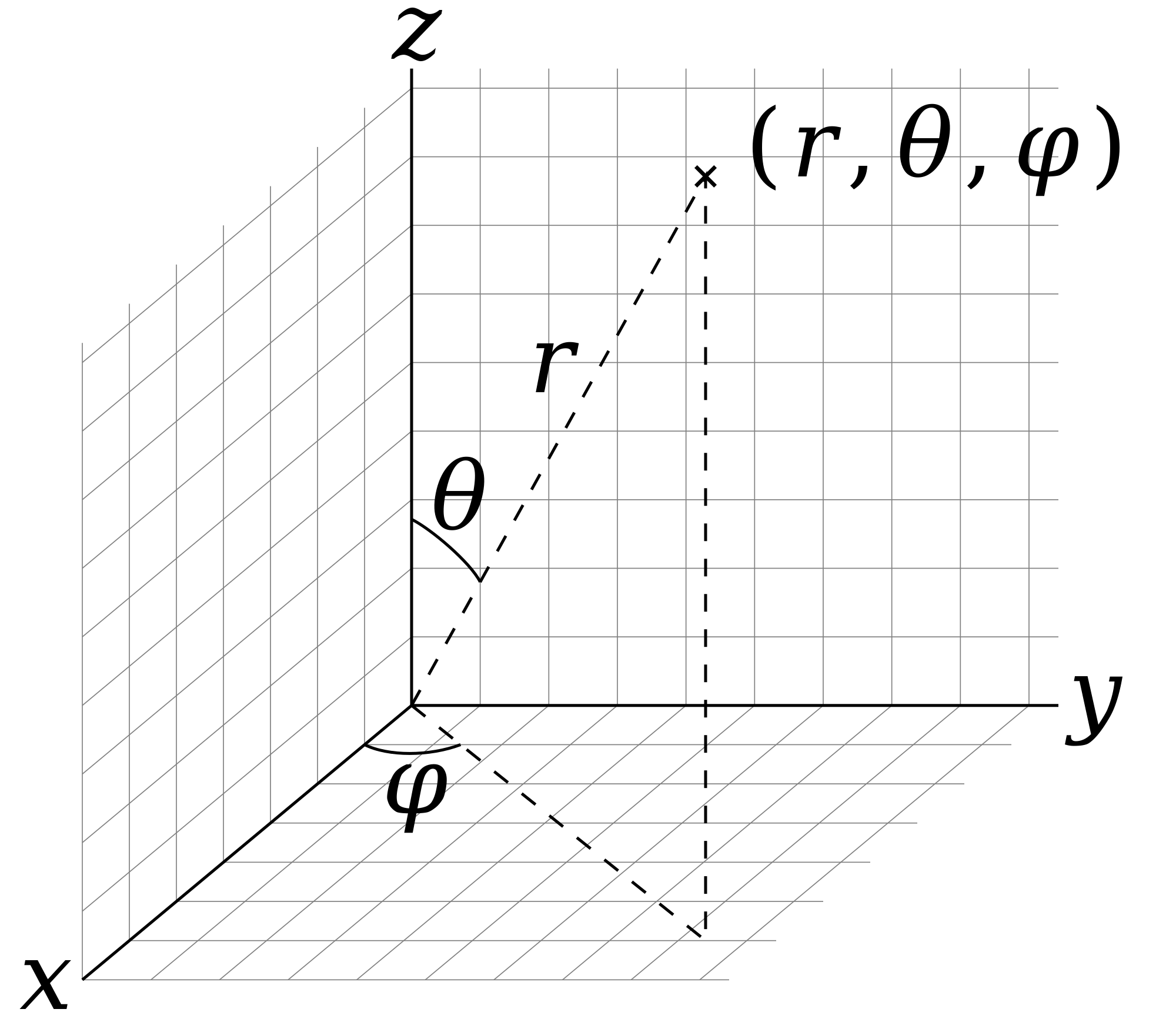
There are two common methods for extending the polar coordinate system to three dimensions. In the cylindrical coordinate system, a z-coordinate with the same meaning as in Cartesian coordinates is added to the r and θ polar coordinates giving a triple (r, θ, z).[8] Spherical coordinates take this a step further by converting the pair of cylindrical coordinates (r, z) to polar coordinates (ρ, φ) giving a triple (ρ, θ, φ).[9]
Homogeneous coordinate system
[edit]A point in the plane may be represented in homogeneous coordinates by a triple (x, y, z) where x/z and y/z are the Cartesian coordinates of the point.[10] This introduces an "extra" coordinate since only two are needed to specify a point on the plane, but this system is useful in that it represents any point on the projective plane without the use of infinity. In general, a homogeneous coordinate system is one where only the ratios of the coordinates are significant and not the actual values.
Other commonly used systems
[edit]Some other common coordinate systems are the following:
- Curvilinear coordinates are a generalization of coordinate systems generally; the system is based on the intersection of curves.
- Orthogonal coordinates: coordinate surfaces meet at right angles
- Skew coordinates: coordinate surfaces are not orthogonal
- The log-polar coordinate system represents a point in the plane by the logarithm of the distance from the origin and an angle measured from a reference line intersecting the origin.
- Plücker coordinates are a way of representing lines in 3D Euclidean space using a six-tuple of numbers as homogeneous coordinates.
- Generalized coordinates are used in the Lagrangian treatment of mechanics.
- Canonical coordinates are used in the Hamiltonian treatment of mechanics.
- Barycentric coordinate system as used for ternary plots and more generally in the analysis of triangles.
- Trilinear coordinates are used in the context of triangles.
There are ways of describing curves without coordinates, using intrinsic equations that use invariant quantities such as curvature and arc length. These include:
- The Whewell equation relates arc length and the tangential angle.
- The Cesàro equation relates arc length and curvature.
Coordinates of geometric objects
[edit]Coordinates systems are often used to specify the position of a point, but they may also be used to specify the position of more complex figures such as lines, planes, circles or spheres. For example, Plücker coordinates are used to determine the position of a line in space.[11] When there is a need, the type of figure being described is used to distinguish the type of coordinate system, for example the term line coordinates is used for any coordinate system that specifies the position of a line.
It may occur that systems of coordinates for two different sets of geometric figures are equivalent in terms of their analysis. An example of this is the systems of homogeneous coordinates for points and lines in the projective plane. The two systems in a case like this are said to be dualistic. Dualistic systems have the property that results from one system can be carried over to the other since these results are only different interpretations of the same analytical result; this is known as the principle of duality.[12]
Transformations
[edit]There are often many different possible coordinate systems for describing geometrical figures. The relationship between different systems is described by coordinate transformations, which give formulas for the coordinates in one system in terms of the coordinates in another system. For example, in the plane, if Cartesian coordinates (x, y) and polar coordinates (r, θ) have the same origin, and the polar axis is the positive x axis, then the coordinate transformation from polar to Cartesian coordinates is given by x = r cosθ and y = r sinθ.
With every bijection from the space to itself two coordinate transformations can be associated:
- Such that the new coordinates of the image of each point are the same as the old coordinates of the original point (the formulas for the mapping are the inverse of those for the coordinate transformation)
- Such that the old coordinates of the image of each point are the same as the new coordinates of the original point (the formulas for the mapping are the same as those for the coordinate transformation)
For example, in 1D, if the mapping is a translation of 3 to the right, the first moves the origin from 0 to 3, so that the coordinate of each point becomes 3 less, while the second moves the origin from 0 to −3, so that the coordinate of each point becomes 3 more.
Coordinate lines/curves
[edit]
Given a coordinate system, if one of the coordinates of a point varies while the other coordinates are held constant, then the resulting curve is called a coordinate curve. If a coordinate curve is a straight line, it is called a coordinate line. A coordinate system for which some coordinate curves are not lines is called a curvilinear coordinate system.[13] Orthogonal coordinates are a special but extremely common case of curvilinear coordinates.
A coordinate line with all other constant coordinates equal to zero is called a coordinate axis, an oriented line used for assigning coordinates. In a Cartesian coordinate system, all coordinates curves are lines, and, therefore, there are as many coordinate axes as coordinates. Moreover, the coordinate axes are pairwise orthogonal.
A polar coordinate system is a curvilinear system where coordinate curves are lines or circles. However, one of the coordinate curves is reduced to a single point, the origin, which is often viewed as a circle of radius zero. Similarly, spherical and cylindrical coordinate systems have coordinate curves that are lines, circles or circles of radius zero.
Many curves can occur as coordinate curves. For example, the coordinate curves of parabolic coordinates are parabolas.
Coordinate planes/surfaces
[edit]

In three-dimensional space, if one coordinate is held constant and the other two are allowed to vary, then the resulting surface is called a coordinate surface. For example, the coordinate surfaces obtained by holding ρ constant in the spherical coordinate system are the spheres with center at the origin. In three-dimensional space the intersection of two coordinate surfaces is a coordinate curve. In the Cartesian coordinate system we may speak of coordinate planes. Similarly, coordinate hypersurfaces are the (n − 1)-dimensional spaces resulting from fixing a single coordinate of an n-dimensional coordinate system.[14]
Coordinate maps
[edit]The concept of a coordinate map, or coordinate chart is central to the theory of manifolds. A coordinate map is essentially a coordinate system for a subset of a given space with the property that each point has exactly one set of coordinates. More precisely, a coordinate map is a homeomorphism from an open subset of a space X to an open subset of Rn.[15] It is often not possible to provide one consistent coordinate system for an entire space. In this case, a collection of coordinate maps are put together to form an atlas covering the space. A space equipped with such an atlas is called a manifold and additional structure can be defined on a manifold if the structure is consistent where the coordinate maps overlap. For example, a differentiable manifold is a manifold where the change of coordinates from one coordinate map to another is always a differentiable function.
Orientation-based coordinates
[edit]In geometry and kinematics, coordinate systems are used to describe the (linear) position of points and the angular position of axes, planes, and rigid bodies.[16] In the latter case, the orientation of a second (typically referred to as "local") coordinate system, fixed to the node, is defined based on the first (typically referred to as "global" or "world" coordinate system). For instance, the orientation of a rigid body can be represented by an orientation matrix, which includes, in its three columns, the Cartesian coordinates of three points. These points are used to define the orientation of the axes of the local system; they are the tips of three unit vectors aligned with those axes.
Geographic systems
[edit]The Earth as a whole is one of the most common geometric spaces requiring the precise measurement of location, and thus coordinate systems. Starting with the Greeks of the Hellenistic period, a variety of coordinate systems have been developed based on the types above, including:
- Geographic coordinate system, the spherical coordinates of latitude and longitude
- Projected coordinate systems, including thousands of cartesian coordinate systems, each based on a map projection to create a planar surface of the world or a region.
- Geocentric coordinate system, a three-dimensional cartesian coordinate system that models the earth as an object, and are most commonly used for modeling the orbits of satellites, including the Global Positioning System and other satellite navigation systems.
See also
[edit]- Absolute angular momentum
- Alphanumeric grid
- Axes conventions in engineering
- Celestial coordinate system
- Coordinate frame
- Coordinate-free
- Fractional coordinates
- Frame of reference
- Galilean transformation
- Grid reference
- Nomogram, graphical representations of different coordinate systems
- Reference system
- Rotation of axes
- Translation of axes
Relativistic coordinate systems
[edit]References
[edit]Citations
[edit]- ^ Woods p. 1
- ^ Weisstein, Eric W. "Coordinate System". MathWorld.
- ^ Weisstein, Eric W. "Coordinates". MathWorld.
- ^ Stewart, James B.; Redlin, Lothar; Watson, Saleem (2008). College Algebra (5th ed.). Brooks Cole. pp. 13–19. ISBN 978-0-495-56521-5.
- ^ Anton, Howard; Bivens, Irl C.; Davis, Stephen (2021). Calculus: Multivariable. John Wiley & Sons. p. 657. ISBN 978-1-119-77798-4.
- ^ Moon P, Spencer DE (1988). "Rectangular Coordinates (x, y, z)". Field Theory Handbook, Including Coordinate Systems, Differential Equations, and Their Solutions (corrected 2nd, 3rd print ed.). New York: Springer-Verlag. pp. 9–11 (Table 1.01). ISBN 978-0-387-18430-2.
- ^ Finney, Ross; George Thomas; Franklin Demana; Bert Waits (June 1994). Calculus: Graphical, Numerical, Algebraic (Single Variable Version ed.). Addison-Wesley Publishing Co. ISBN 0-201-55478-X.
- ^ Margenau, Henry; Murphy, George M. (1956). The Mathematics of Physics and Chemistry. New York City: D. van Nostrand. p. 178. LCCN 55010911. OCLC 3017486.
- ^ Morse, PM; Feshbach, H (1953). Methods of Theoretical Physics, Part I. New York: McGraw-Hill. p. 658. LCCN 52011515.
- ^ Jones, Alfred Clement (1912). An Introduction to Algebraical Geometry. Clarendon.
- ^ Hodge, W.V.D.; D. Pedoe (1994) [1947]. Methods of Algebraic Geometry, Volume I (Book II). Cambridge University Press. ISBN 978-0-521-46900-5.
- ^ Woods p. 2
- ^ Tang, K. T. (2006). Mathematical Methods for Engineers and Scientists. Vol. 2. Springer. p. 13. ISBN 3-540-30268-9.
- ^ Liseikin, Vladimir D. (2007). A Computational Differential Geometry Approach to Grid Generation. Springer. p. 38. ISBN 978-3-540-34235-9.
- ^ Munkres, James R. (2000) Topology. Prentice Hall. ISBN 0-13-181629-2.
- ^ Hanspeter Schaub; John L. Junkins (2003). "Rigid body kinematics". Analytical Mechanics of Space Systems. American Institute of Aeronautics and Astronautics. p. 71. ISBN 1-56347-563-4.
Sources
[edit]- Voitsekhovskii, M.I.; Ivanov, A.B. (2001) [1994], "Coordinates", Encyclopedia of Mathematics, EMS Press
- Woods, Frederick S. (1922). Higher Geometry. Ginn and Co. pp. 1ff.
- Shigeyuki Morita; Teruko Nagase; Katsumi Nomizu (2001). Geometry of Differential Forms. AMS Bookstore. p. 12. ISBN 0-8218-1045-6.
External links
[edit]| International | |
|---|---|
| National | |
| Other | |
Coordinate system
View on GrokipediaFundamental concepts
Definition and purpose
A coordinate system originated with the work of René Descartes in his 1637 treatise La Géométrie, where he introduced a method to link algebraic equations with geometric figures, thereby founding analytic geometry and enabling the numerical description of spatial positions.[7] This innovation allowed geometric problems to be solved using algebraic techniques, marking a shift from purely synthetic methods to those incorporating coordinates. In mathematics, a coordinate system is defined as a systematic way to assign to each point in a space a unique tuple of numbers, typically from the real numbers or another field, relative to a chosen reference frame.[8] This mapping function facilitates the precise identification and manipulation of positions within Euclidean spaces, abstract vector spaces, or even infinite-dimensional settings like function spaces, where points correspond to functions and coordinates to basis expansions.[9] The primary purpose of coordinate systems is to enable quantitative analysis in geometry, physics, and computation, such as calculating distances, angles, and transformations between points or objects.[1] They provide a framework for modeling physical phenomena, from particle trajectories in mechanics to data representations in algorithms, by converting qualitative spatial relations into operable numerical forms. For instance, the Cartesian coordinate system serves as a foundational example, using perpendicular axes to assign (x, y) or (x, y, z) values.[10] Prior to coordinate systems, geometry relied on synthetic approaches—using axioms, postulates, and constructions without numerical assignments—as in Euclid's Elements, which emphasized intrinsic properties like congruence and similarity.[7] Coordinate methods, by contrast, require algebraic prerequisites but unlock computational power, allowing proofs and predictions through equations rather than diagrams alone.[11]Coordinate tuples and spaces
In mathematics, a coordinate tuple, also known as a coordinate vector, is an ordered n-tuple of scalars that uniquely identifies the position of a point within an n-dimensional space, typically over the field of real numbers or more generally over any field such as the complex numbers .[12] This tuple establishes a bijection between points in the space and elements of the corresponding vector space, allowing abstract geometric objects to be represented numerically for computation and analysis.[13] Coordinate tuples are defined relative to an ambient space, which provides the underlying structure for their interpretation; common examples include Euclidean spaces equipped with an inner product, affine spaces without a designated origin but with parallel translation, and metric spaces where distances are preserved. In such spaces, the tuple is referenced to a fixed origin (a point designated as the zero vector) and a basis consisting of linearly independent vectors that span the space, enabling the decomposition of any position vector as a linear combination , where are the basis vectors.[14] The choice of basis influences the form of the coordinates: orthogonal coordinates employ perpendicular basis vectors (with for ), simplifying calculations involving distances and angles via the Pythagorean theorem, whereas oblique coordinates use non-perpendicular basis vectors, which may arise in skewed or sheared representations but require a metric tensor to compute inner products.[15] In curvilinear coordinate systems, which generalize rectilinear ones by allowing curved coordinate lines, the coordinate basis vectors are defined as the partial derivatives of the position vector with respect to each coordinate , yielding ; these basis vectors are generally neither orthogonal nor of unit length, necessitating scale factors for normalization.[16] The dimensionality of coordinate spaces varies: zero-dimensional spaces consist of isolated points representable by an empty tuple, one-dimensional cases by a single scalar, and higher finite dimensions by corresponding n-tuples, while infinite-dimensional spaces, such as separable Hilbert spaces, use countable infinite tuples or series expansions in an orthonormal basis to represent elements with square-summable coefficients, enabling applications in functional analysis.[12][17]Low-dimensional coordinate systems
Number line
The number line represents the foundational one-dimensional coordinate system, consisting of the set of all real numbers arranged sequentially along a straight line. The origin is designated at the point corresponding to 0, with numbers increasing in the positive direction to the right and decreasing in the negative direction to the left./01%3A_Real_Numbers_and_Their_Operations/1.01%3A_Real_numbers_and_the_Number_Line)[18] A position on the number line is specified by a single real number , which denotes the signed distance from the origin. This signed distance measures the displacement along the line, where a positive value indicates a location to the right of the origin and a negative value to the left, with the magnitude giving the absolute distance.[18]/01%3A_Real_Numbers_and_Their_Operations/1.01%3A_Real_numbers_and_the_Number_Line) The number line finds essential applications in parameterizing time, as in classical physics where time quantifies progression from an initial reference point along a continuous timeline.[19] It also underpins basic measurement scales, such as linear rulers for distance or uniform thermometers for temperature, enabling precise quantification of magnitudes in one dimension.[20] Extensions of the number line include directed line segments, which incorporate both length and orientation from an initial point to an endpoint, facilitating the representation of displacements with direction in one dimension.[21] A variant arises in modular arithmetic, where the line is conceptualized as a circle to model periodic wrapping, such as clock hours modulo 12, preserving one-dimensional positioning but with bounded repetition.[22]Cartesian coordinate system
The Cartesian coordinate system is an orthogonal coordinate system that specifies the position of points in Euclidean space using ordered tuples of real numbers, each representing the signed distance from a reference point along perpendicular axes. This system, introduced by René Descartes in his 1637 work La Géométrie, enables the algebraic representation of geometric objects and forms the foundation of analytic geometry.[7] In an n-dimensional Euclidean space, the Cartesian coordinate system is constructed by selecting n mutually perpendicular axes that intersect at a common origin point O. Each point P in the space is identified by an ordered tuple of coordinates (x₁, x₂, ..., xₙ), where xᵢ denotes the projection of the vector from O to P onto the i-th axis, measured as a signed distance along that axis, akin to positioning on a number line.[23][24] In two dimensions, the system uses a plane with two perpendicular axes labeled x and y intersecting at the origin, allowing points to be represented as (x, y). In three dimensions, it extends to a space with three mutually perpendicular axes x, y, and z, where points are denoted (x, y, z); the axes typically follow a right-handed orientation, such that rotating from the positive x-axis to the positive y-axis aligns the thumb of the right hand with the positive z-axis.[24][25] The metric properties of the Cartesian system derive from the Euclidean metric, enabling direct computation of distances and angles. The Euclidean distance d between two points with coordinates (x₁, ..., xₙ) and (y₁, ..., yₙ) is given by which represents the length of the straight-line segment connecting them.[26] The inner product of two vectors u = (u₁, ..., uₙ) and v = (v₁, ..., vₙ), which measures their alignment and is foundational for orthogonality, is defined as This inner product yields the squared distance when applied to the difference vector and supports the system's orthogonality, as the basis vectors along each axis have an inner product of zero with one another.[27][28] Applications of the Cartesian coordinate system are central to analytic geometry, where geometric problems are solved algebraically by representing curves and surfaces via equations in coordinates. It also underpins basic vector calculus, facilitating operations like differentiation and integration in Euclidean spaces for modeling physical phenomena such as motion and fields.[28]Curvilinear coordinate systems
Polar coordinate system
The polar coordinate system is a two-dimensional curvilinear coordinate system that specifies the position of a point in the plane using two values: the radial distance from a fixed origin (called the pole) and the angle measured counterclockwise from the positive x-axis (the polar axis).[29] Here, represents the distance from the pole, while is typically expressed in radians (with a range of ) or degrees (with a range of ), though angles differing by multiples of radians describe the same point. This system is particularly suited for describing phenomena with rotational symmetry, such as orbits or waves emanating from a central point.[30] To relate polar coordinates to the Cartesian system, the transformation equations are and , which project the point onto the rectangular axes.[29] Conversely, converting from Cartesian to polar coordinates yields and , where the two-argument arctangent function accounts for the correct quadrant based on the signs of and .[29] These conversions leverage the definitions of sine and cosine in the unit circle, ensuring a one-to-one correspondence except at the origin, where for any . In the polar system, the infinitesimal line element that measures distances is given by , derived from the Pythagorean theorem in the local tangent frame.[31] This metric corresponds to orthogonal scale factors for the radial direction and for the angular direction, indicating that angular displacements scale with the distance from the origin.[31] These factors facilitate computations in vector calculus, such as gradients or integrals over regions with circular boundaries.[32] Polar coordinates find essential applications in describing circular motion, where the constant radius simplifies the kinematics of objects like planets or pendulums, reducing equations to angular variables.[33] In complex analysis, they represent complex numbers as , enabling elegant handling of multiplication, exponentiation, and rotations via properties of the exponential function.[34] This form underscores the system's utility in fields like signal processing and quantum mechanics for modeling periodic phenomena.[34]Cylindrical and spherical coordinate systems
Cylindrical coordinates extend the two-dimensional polar coordinate system into three dimensions by incorporating a vertical coordinate along the axis of symmetry. In this system, a point in space is specified by the tuple , where represents the radial distance from the z-axis (with ), is the azimuthal angle measured from the positive x-axis in the xy-plane (ranging from 0 to ), and is the height along the z-axis (extending from to ).[35] The transformation to Cartesian coordinates is given by The line element, or infinitesimal distance , in cylindrical coordinates is which reflects the orthogonal nature of the coordinate surfaces: cylinders of constant , planes of constant , and planes of constant .[36] Spherical coordinates provide a system suited for describing positions relative to a central origin in three-dimensional space, using radial distance and two angular coordinates. A point is denoted by , where is the radial distance from the origin (), is the polar angle from the positive z-axis (ranging from 0 to ), and is the azimuthal angle in the xy-plane (from 0 to ).[37] The corresponding Cartesian conversions are The line element in spherical coordinates is accounting for the geometry of spheres of constant , cones of constant , and planes of constant .[36] In both systems, scale factors arise from the metric tensor components, influencing integrals over volumes and surfaces. For cylindrical coordinates, the volume element is , where the factor accounts for the increasing circumference at larger radii.[38] In spherical coordinates, the volume element is , with deriving from the surface area of spherical shells and the varying latitude-dependent arc length.[39] These coordinate systems find prominent applications in physical contexts exhibiting cylindrical or spherical symmetry. Cylindrical coordinates are particularly useful in electromagnetism for problems involving long straight wires or coaxial cables, where the axial symmetry simplifies the expressions for fields like the magnetic field around a current-carrying wire.[40] Spherical coordinates are essential in gravitational studies, such as modeling the potential around spherical masses like planets or stars, enabling the use of spherical harmonics to expand the gravitational field in terms of angular dependencies.[41]Higher-dimensional and projective systems
Homogeneous coordinate system
A homogeneous coordinate system extends the representation of points from affine space to projective space by incorporating an additional coordinate dimension, allowing for a unified treatment of points at infinity and perspective transformations. In an n-dimensional projective space , a point is represented by an equivalence class of -tuples , where two tuples are equivalent if one is a scalar multiple of the other by , denoted as .[42] This scale invariance ensures that the representation is projective rather than metric.[43] To recover affine coordinates from homogeneous ones, dehomogenization divides the first components by the last when , yielding .[44] In two dimensions, for example, the homogeneous tuple corresponds to the Cartesian point in the affine plane, while tuples with , such as , represent points at infinity, which model directions or vanishing points without a finite position.[45] The Cartesian coordinate system thus forms the affine subset of the projective plane where the homogeneous coordinate .[46] Transformations in homogeneous coordinates are linear and represented by matrices acting on the tuples, preserving the equivalence relation and thus the projective structure; these are defined up to scalar multiplication and include the full group of projective transformations. Such transformations maintain cross-ratios, a key projective invariant that generalizes ratios in affine geometry. For perspective projection, a common operation maps 3D points to 2D images via a matrix that incorporates the camera's focal length and position, effectively handling the convergence of parallel lines at infinity.[47] In applications, homogeneous coordinates are essential in computer graphics for efficient handling of perspective projections and viewport transformations, as seen in rendering pipelines like those in OpenGL.[48] They enable ray tracing by parameterizing rays as lines in projective space, simplifying intersections with objects at varying depths.[49] In robotics and computer vision, they model pinhole camera projections, where 3D world points are mapped to 2D image coordinates, facilitating tasks like pose estimation and multi-view reconstruction.Other commonly used systems
Toroidal coordinates provide a three-dimensional orthogonal curvilinear system well-suited for regions with toroidal symmetry, such as doughnut-shaped domains. Defined by parameters (σ, τ, φ), the coordinate surfaces consist of confocal tori (σ = constant), spheres (τ = constant), and meridional planes (φ = constant). The relation to Cartesian coordinates is where is a scale parameter representing the distance from the origin to the degenerate torus (the ring circle). The line element is These coordinates facilitate solving partial differential equations like Laplace's equation in toroidal geometries, with applications in electromagnetism for modeling fields around ring currents or tokamak plasmas.[50][51] Elliptic coordinates extend to two and three dimensions, employing confocal ellipses and hyperbolae as coordinate curves to address problems with elliptical symmetry. In 2D, parameters (μ, ν) yield where is half the focal distance, with μ = constant tracing ellipses and ν = constant tracing hyperbolae. The scale factors are , giving the metric In 3D, elliptic cylindrical coordinates append a z-direction, while prolate/oblate spheroidal variants adapt for ellipsoidal foci. Laplace's equation separates in these coordinates, enabling exact solutions for boundary value problems in elliptic domains, such as heat conduction or electrostatics in elliptical waveguides.[52][51] Parabolic coordinates form another orthogonal curvilinear system, ideal for domains bounded by confocal parabolas. In 2D, using (σ, τ) with σ ≥ 0, τ ∈ ℝ, where σ = constant and τ = constant define families of parabolas opening in opposite directions. The metric is The 3D version incorporates an azimuthal angle φ, yielding These coordinates simplify solutions to Laplace's equation for parabolic reflectors or flows, as seen in optics and fluid dynamics. Other systems like bispherical coordinates, which use confocal spheres and planes with metric , extend orthogonality to spherical symmetries beyond standard spherical coordinates.[51] Bipolar coordinates, based on two fixed foci, offer a 2D orthogonal system for geometries involving circular or cylindrical boundaries centered on dual points. For foci at (±a, 0), parameters (τ, σ) satisfy τ = artanh(y / (x + \sqrt{x^2 + y^2})), but commonly, τ measures the logarithmic distance ratio to the foci, and σ the angular separation. The transformation is with metric In potential theory, they enable separable solutions for Laplace's equation around two poles, such as electrostatic potentials between coaxial cylinders or spheres, simplifying capacitance calculations. The 3D bipolar cylindrical extension adds a z-coordinate for axial symmetry.[53][51]Representation of geometric objects
Coordinates of points and vectors
In a coordinate system, a point is represented by an ordered tuple of real numbers, known as its coordinates, which quantify its position relative to a designated origin and a set of basis directions. These coordinates provide an absolute positioning when measured from a fixed origin, but relative positioning between two points can be determined by subtracting their coordinate tuples, yielding the components of a displacement vector.[54] Vectors, which encode directed quantities such as displacement or velocity, are mathematically defined as the difference between the position vectors of two points in the system.[55] In a given basis , a vector is expressed as , where the scalars are its components along each basis vector.[56] The magnitude of , denoted , is computed as , with representing the inner product; in an orthonormal basis, this simplifies to .[55] For example, in a three-dimensional Cartesian coordinate system with orthonormal basis vectors , , , a point has coordinates , corresponding to the position vector , while a vector is represented as .[57] Vectors are classified as free or bound: free vectors depend only on magnitude and direction, allowing translation without alteration, whereas bound vectors are fixed at a specific point of application.[58] In curvilinear coordinate systems, where basis vectors vary with position, vectors are decomposed into components relative to local tangent vectors, which are derived as partial derivatives of the position function with respect to the coordinates.[59] These tangent vectors lie along the coordinate curves and form a position-dependent basis, enabling the representation of vectors at each point while preserving directional and magnitude properties through the inner product.Coordinates of lines, curves, and surfaces
In coordinate geometry, lines are fundamental one-dimensional objects that can be represented parametrically using a point and a direction vector. The parametric equation of a line passing through a point in the direction of a nonzero vector is given by , where is a scalar parameter ranging over the real numbers.[60] This form extends the concept of points by incorporating a linear progression along the direction vector. An equivalent representation, known as the two-point form, describes the line passing through two distinct points and in the plane as , assuming .[61] In two dimensions, lines can also be expressed in normal form as , where is a normal vector to the line and determines its position relative to the origin.[62] Curves in three-dimensional space extend this parameterization to more general paths. A space curve can be represented parametrically as , where , , and are differentiable functions of the parameter , tracing the locus of points as varies over an interval.[63] For analyzing geometric properties independent of the parameterization speed, curves are often reparameterized by arc length , where measures the distance along the curve from an initial point, yielding a unit-speed parameterization with ./13%3A_Vector-Valued_Functions/13.03%3A_Arc_Length_and_Curvature) Surfaces, as two-dimensional extensions, require two parameters for their coordinate representation. A parametric surface is defined by , where and vary over a domain in the plane, mapping to points on the surface in three-dimensional space.[64] Alternatively, surfaces can be described implicitly by an equation , where is a continuous function whose level set at zero forms the surface, useful for defining boundaries without explicit parameterization.[65] For space curves parameterized by arc length, the Frenet-Serret apparatus provides a local orthogonal frame consisting of the unit tangent vector , the principal normal , and the binormal . The evolution of this frame is governed by the Frenet-Serret formulas: where is the curvature, measuring the rate of turning of the tangent, and is the torsion, quantifying the twisting out of the osculating plane.[66] These relations, originally derived by Frenet in his 1847 thesis and independently by Serret in 1851, form the foundation for intrinsic curve analysis in differential geometry.[67]Transformations between systems
Change of coordinates
A change of coordinates refers to the process of mapping points from one coordinate system to another through a smooth invertible function, known as a diffeomorphism. In the context of manifolds, if two charts (U, φ) and (V, ψ) overlap on a manifold M, the transition map φ ∘ ψ⁻¹: ψ(U ∩ V) → φ(U ∩ V) is a diffeomorphism between open subsets of Euclidean space, ensuring compatibility and smoothness across the systems. This mapping allows expressions of geometric objects to be transferred between systems while preserving topological and differentiable structure.[68][69] Changes of coordinates can be distinguished as active or passive transformations. A passive transformation relabels points by altering the coordinate axes or basis without moving the physical points themselves, effectively changing the description of a fixed configuration. In contrast, an active transformation displaces the points in space while keeping the coordinate system fixed, such as rotating an object to a new position. This distinction is crucial in applications like relativity and mechanics, where passive views emphasize coordinate invariance.[70] Under a change of coordinates, the components of vectors and tensors adjust to maintain their intrinsic properties, leading to contravariant and covariant transformation rules. Contravariant vector components transform asreflecting how they scale inversely to basis changes, while covariant vector components transform as
with the basis covectors transforming contravariantly as
These rules ensure that the contraction V^i W_i remains invariant.[71] Covariant components transform like basis vectors, which vary as
emphasizing their "co-varying" nature.[72] In Cartesian coordinates, a common example is a rotation, where the passive transformation matrix for a counterclockwise rotation by angle θ in 2D is
relabeling axes to express the same points in the rotated frame.[73] For curvilinear systems, such as transitioning to polar coordinates, scale adjustments via factors like h_φ = r account for varying distances along curved lines, ensuring accurate representation of lengths and ensuring the metric tensor adapts properly during the mapping.[31] The Jacobian matrix of the diffeomorphism provides a brief reference for how local volumes scale under these changes.
Jacobian matrix and determinant
The Jacobian matrix arises in the context of differentiable coordinate transformations between systems, serving as the matrix of first-order partial derivatives that linearizes the mapping locally. For a transformation from coordinates to , the Jacobian matrix is defined as where the entries are the partial derivatives of the new coordinates with respect to the old ones. This matrix captures how infinitesimal changes in the original coordinates propagate to the transformed system, approximating the transformation as a linear map near a point.[74] Key properties of the Jacobian matrix include its behavior under composition of transformations and the role of its determinant in preserving geometric structure. By the multivariable chain rule, the Jacobian of a composite transformation is the product of the individual Jacobians: .[75] The determinant indicates scaling and orientation: if , the transformation preserves local orientation, while reverses it; a zero determinant signals a singularity where the transformation is not locally invertible. In applications to integration, the Jacobian determinant enables the change of variables formula for multiple integrals over regions in . Specifically, for a diffeomorphism , which accounts for the distortion of volume elements under the mapping, with the absolute value ensuring positive measure. This is essential for evaluating integrals in convenient coordinates, such as simplifying bounds or exploiting symmetry, and singularities (where ) identify points where the transformation fails to cover the space properly, potentially requiring careful handling of the domain.[74] In curvilinear coordinate systems, the Jacobian relates to the metric tensor, which defines distances and angles intrinsically. For a parametrization of the space, the metric tensor components are forming the Gram matrix of the tangent vectors, which are columns of the Jacobian matrix of with respect to the parameters.[76] The determinant of the metric tensor, , gives the volume scaling factor, analogous to in the transformation context, and facilitates computations like line elements .[76]Structural components
Coordinate lines and curves
In a coordinate system defined by coordinates , coordinate lines, also known as coordinate curves, are the one-dimensional paths traced by varying a single coordinate while holding all other coordinates fixed. These lines are integral curves of the coordinate basis vectors and lie tangent to at each point along the path.[77][78] In curvilinear coordinate systems, such as those used in non-Euclidean or adapted geometries, coordinate lines are generally curved and do not coincide with geodesics unless the system is specially chosen. The infinitesimal arc length along a coordinate line for is given by , where the scale factor accounts for the local stretching or compression of the coordinate, with denoting the position vector. The total length of such a line segment is then .[79][78] For orthogonal curvilinear coordinates, the coordinate lines associated with different indices intersect at right angles everywhere, simplifying metric computations as the line element becomes . A classic example is the two-dimensional polar coordinate system , where the coordinate lines for fixed are straight radial rays emanating from the origin, and those for fixed are concentric circular arcs; here, and , so the length along a radial line is simply while along a circular arc it is .[80]Coordinate planes and surfaces
In three-dimensional Cartesian coordinates, the coordinate planes are the hypersurfaces obtained by fixing one coordinate to a constant value. For instance, fixing the z-coordinate at a constant k yields the plane z = k, which is parallel to the xy-plane; similarly, x = k defines a plane parallel to the yz-plane, and y = k a plane parallel to the xz-plane. These planes, along with the principal coordinate planes (x=0, y=0, z=0), form the fundamental grid that divides Euclidean space into octants and provides a basis for visualizing and solving problems in vector calculus and physics.[81] In curvilinear coordinate systems, such as spherical coordinates (ρ, θ, φ), where ρ is the radial distance, θ the azimuthal angle, and φ the polar angle, the coordinate surfaces are more varied geometrically. Fixing ρ = constant produces spheres centered at the origin; fixing θ = constant results in vertical half-planes containing the z-axis; and fixing φ = constant generates cones with apex at the origin and axis along the z-axis, such as φ = π/4 forming a 45-degree cone. The metric induced on these surfaces, derived from the ambient Euclidean metric, governs distances and areas within them—for example, on a cone φ = constant, the induced metric simplifies to ds² = dρ² + ρ² sin² φ dθ², reflecting the conical geometry.[37][82] In n-dimensional Euclidean space, coordinate hypersurfaces are (n-1)-dimensional submanifolds obtained by fixing one coordinate to a constant, generalizing the planes in 3D. For example, in Cartesian coordinates (x₁, ..., xₙ), fixing xᵢ = c defines a hyperplane parallel to the other coordinate axes, forming an affine subspace of dimension n-1. These hypersurfaces foliate the space, partitioning it into layers that facilitate integration, change of variables, and analysis of multidimensional functions. In curvilinear systems, such fixed-coordinate sets yield more complex hypersurfaces, like hypercones or hyperspheres, with induced metrics that account for the curvature of the coordinate grid.[83] Coordinate planes and hypersurfaces play key roles in applications, such as dividing space into regions for domain decomposition in numerical methods or serving as boundaries in partial differential equations (PDEs). In PDEs, like the Laplace equation ∇²u = 0 on a rectangular domain, boundary conditions are often specified on coordinate planes (e.g., Dirichlet conditions u=0 on x=0 and x=a), enabling separation of variables and exact solutions via Fourier series. This structure simplifies solving heat conduction or electrostatic problems in bounded regions.[84]Coordinate systems in geometry and topology
Coordinate maps and charts
In differential geometry, a coordinate map, also known as a coordinate chart, provides a local representation of a manifold by mapping an open subset of the manifold to an open subset of Euclidean space. Specifically, for an n-dimensional manifold M, a coordinate chart is a pair (U, φ), where U is an open subset of M and φ: U → ℝ^n is a bijective continuous map with a continuous inverse, making φ a homeomorphism onto its image φ(U), which is open in ℝ^n. This structure allows points on the manifold to be assigned local coordinates in a way that resembles Euclidean space, facilitating the application of calculus and analysis.[85] For smooth manifolds, the coordinate map must satisfy additional regularity conditions to ensure compatibility with the smooth structure. The map φ is required to be a diffeomorphism, meaning both φ and its inverse φ^{-1} are infinitely differentiable (smooth) functions. Moreover, if two coordinate charts (U, φ) and (V, ψ) on M have overlapping domains (U ∩ V ≠ ∅), the transition map ψ ∘ φ^{-1}: φ(U ∩ V) → ψ(U ∩ V) must be smooth, ensuring that the local coordinate representations are compatible across overlaps. The domain U is open in the topology induced on M, and this setup defines the maximal smooth atlas on M.[86] The regularity of a coordinate map is further characterized by the properties of its differential dφ. At each point x ∈ U, the linear map dφ_x: T_x M → T_{φ(x)} ℝ^n must have full rank n, meaning it is both injective (making φ an immersion) and surjective (making φ a submersion) locally. This full-rank condition guarantees that φ is a local diffeomorphism, preserving the dimension and smoothness of the manifold structure without singularities. Such regularity ensures that tangent spaces and differential forms can be consistently transferred between the manifold and Euclidean space via the chart. A classic example of a coordinate map is the stereographic projection on the 2-sphere S^2. Consider the projection from the north pole (0,0,1) onto the xy-plane: for a point p = (x,y,z) ∈ S^2 excluding the north pole, the map φ(p) = (x/(1-z), y/(1-z)) ∈ ℝ^2 is a diffeomorphism, providing coordinates that cover S^2 minus one point. A second chart from the south pole covers the remaining point, and their transition map is smooth, illustrating how coordinate maps enable a global description of the manifold. Coordinate maps are fundamental building blocks, and collections of them form atlases that cover the entire manifold.[87]Atlases on manifolds
In differential geometry, an atlas on a manifold is a collection of coordinate charts, where each is an open set, is a homeomorphism onto an open subset of Euclidean space, the sets form an open cover of , and the transition maps are smooth (i.e., ) diffeomorphisms on their domains for all .[88] This structure allows local Euclidean coordinates to be glued together globally while preserving differentiability.[89] The compatibility condition ensures that the atlas induces a well-defined smooth structure on , meaning that functions and maps defined using these coordinates behave consistently across overlaps. A smooth atlas is maximal if it contains every compatible chart on ; every smooth atlas extends uniquely to a maximal one, which fully determines the smooth structure and allows the manifold to be equipped with a consistent notion of differentiability.[88] The dimension must be the same for all charts in the atlas, reflecting the intrinsic dimensionality of .[89] For example, the 2-sphere cannot be covered by a single chart diffeomorphic to due to topological obstructions like non-trivial homology, requiring at least two charts—such as stereographic projections from the north and south poles—to form a smooth atlas with compatible transitions near the equator.[88] Similarly, Riemann surfaces, which are one-dimensional complex manifolds (real dimension 2), rely on atlases of holomorphic charts where transition maps are biholomorphic, enabling global definitions of complex-analytic functions; the Riemann sphere, for instance, uses two charts analogous to those on .[90]Specialized applications
Orientation-based coordinates
Orientation-based coordinates describe the spatial orientation of a local coordinate frame relative to a fixed reference frame, typically through parameters that capture rotations in three-dimensional Euclidean space. These systems are essential in fields where the alignment of material structures or rigid bodies must be precisely quantified, such as in crystallography for crystal lattice orientations or in rigid body dynamics for object poses. Unlike position-based coordinates, orientation-based ones focus solely on rotational degrees of freedom, parameterizing the special orthogonal group SO(3), which consists of all proper rotations in 3D space.[91] A widely used parameterization is Euler angles, denoted as (α, β, γ), which represent a sequence of three successive rotations about specific axes of the coordinate frame. For instance, in the ZYZ convention common in crystallography, the first rotation by α is about the z-axis, followed by β about the new y-axis, and γ about the new z-axis again. This composition yields a rotation matrix , an orthogonal 3×3 matrix with determinant 1 that transforms vectors from the local to the reference frame: where each is a basic rotation matrix. However, Euler angles suffer from gimbal lock, a singularity where the representation loses one degree of freedom—typically when β = ±90°—causing multiple orientations to map to the same point and complicating interpolation or control. This issue arises due to the topological properties of SO(3), which is not simply connected and requires at least three parameters but exhibits such degeneracies in angular representations.[92][93][94] In applications like molecular modeling, Euler angles facilitate the alignment of protein structures or crystal orientations during techniques such as molecular replacement in X-ray crystallography, enabling the computation of rotation matrices to fit models to experimental density maps. Similarly, in aerospace attitude control, they describe the orientation of spacecraft or aircraft relative to inertial frames, aiding in stability analysis and control system design for maneuvers. To mitigate gimbal lock, quaternions serve as an alternative representation, expressed as with , providing a singularity-free mapping from the 4D hypersphere to SO(3) via double covering. Quaternions are particularly valued in these domains for smooth interpolation (slerp) and numerical stability in simulations.[95][96][97]Geographic coordinate systems
Geographic coordinate systems provide a standardized method for specifying locations on Earth's surface, primarily using angular measurements relative to the equator and prime meridian, augmented by a vertical component for three-dimensional positioning. These systems approximate the Earth as an oblate spheroid rather than a perfect sphere to account for its equatorial bulge, enabling precise global navigation and mapping. While often idealized using spherical coordinates for mathematical simplicity, geographic systems incorporate ellipsoidal models to reflect the planet's true shape.[98] In geodetic coordinates, positions are defined by three parameters: geodetic latitude , which measures the angle from the equator toward the poles ranging from at the South Pole to at the North Pole; geodetic longitude , which measures the angle east or west from the prime meridian ranging from to ; and ellipsoidal height , the distance above or below the reference ellipsoid along the local normal.[99] These coordinates form the basis for global positioning, with latitude and longitude providing horizontal location and height adding the vertical dimension.[100] The reference surface for these coordinates is typically an ellipsoid of revolution, defined by its semi-major axis (equatorial radius) and flattening (measure of polar compression). The World Geodetic System 1984 (WGS84), a standard datum used internationally, employs an ellipsoid with m and .[101] This model closely approximates the geoid, an equipotential surface coinciding with mean sea level, but deviates due to local gravitational variations; these deviations, known as geoid undulations, range from approximately m to m relative to the WGS84 ellipsoid.[102] Undulations are critical for converting ellipsoidal heights to orthometric heights (above sea level), ensuring accurate elevation data in applications like surveying.[103] To represent curved geographic coordinates on flat maps, map projections transform the ellipsoidal surface onto a plane, inevitably introducing distortions in shape, area, distance, or direction. The Mercator projection, a cylindrical conformal projection suitable for navigation, maps longitude directly to the x-coordinate and latitude to the y-coordinate via the formula: where angles are in radians and distances are scaled by the ellipsoid's radius.[104] This projection preserves angles (conformal), making it ideal for compass bearings, but it distorts areas progressively toward the poles, exaggerating high-latitude regions like Greenland.[105] Geographic coordinate systems underpin key applications in modern geospatial technology. The Global Positioning System (GPS) relies on WGS84 to broadcast satellite positions and compute user locations in latitude, longitude, and height.[101] In cartography, these coordinates enable the creation of thematic and topographic maps through projections. For regional analysis requiring Cartesian-like grids, the Universal Transverse Mercator (UTM) system projects the ellipsoid onto 60 transverse Mercator zones, each 6° wide in longitude, providing easting and northing values in meters for low-distortion local mapping.[106]Relativistic coordinate systems
In special relativity, coordinate systems are extended to four-dimensional spacetime, incorporating time as a coordinate on equal footing with space to account for the invariance of the speed of light. The standard framework is Minkowski space, where coordinates are typically denoted as (ct, x, y, z), with c being the speed of light, and the spacetime interval is given by the metric [107] This pseudo-Euclidean metric distinguishes timelike, spacelike, and lightlike separations, enabling the description of causal structure in flat spacetime.[107] Transformations between inertial frames in Minkowski space are governed by Lorentz transformations, which preserve the metric; for motion along the x-axis with velocity v, they take the form [108] where .[108] These coordinates reduce to the flat-space limit of Cartesian systems when the speed of light is taken to infinity.[109] Inertial frames in special relativity are those moving at constant velocity relative to one another, where the laws of physics, including Maxwell's equations, take their simplest form without fictitious forces.[109] Non-inertial frames, such as accelerating ones, require additional terms to describe motion, but special relativity applies strictly to inertial observers; extensions to non-inertial cases are handled in general relativity.[110] General relativity generalizes coordinate systems to curved spacetime, where the metric tensor encodes gravitational effects through the equivalence principle, treating acceleration and gravity as locally indistinguishable.[110] A seminal example is the Schwarzschild coordinate system for the exterior of a spherically symmetric, non-rotating mass M, with coordinates (t, r, θ, φ) and metric [111] where G is the gravitational constant; this solution describes the geometry around black holes and stars.[111] However, these coordinates exhibit singularities at r = 0 (a physical curvature singularity) and at r = 2GM/c² (the event horizon), the latter being a coordinate singularity removable by transformations like Kruskal-Szekeres coordinates, indicating no true breakdown of spacetime there.[112] Relativistic coordinate systems find practical applications in technologies like the Global Positioning System (GPS), where satellite clocks experience time dilation: special relativistic effects from orbital velocity cause a daily loss of about 7 μs, while general relativistic gravitational effects cause a gain of about 45 μs, resulting in a net gain of approximately 38 μs per day, necessitating built-in corrections of approximately 38 μs per day for positional accuracy within meters.[113] In cosmology, the Friedmann-Lemaître-Robertson-Walker (FLRW) coordinates describe homogeneous, isotropic expanding universes with metric (for flat space, k=0), where a(t) is the scale factor governing cosmic expansion, originally derived from Einstein's field equations assuming spatial uniformity.References
- https://proofwiki.org/wiki/Definition:Oblique_Coordinate_System