In the era of the old quantum theory, starting from Max Planck's proposal of quanta in his model of blackbody radiation (1900) and Albert Einstein's adaptation of the concept to explain the photoelectric effect (1905), and until Erwin Schrödinger published his eigenfunction equation in 1926,^[1] the concept behind quantum numbers developed based on atomic spectroscopy and theories from classical mechanics with extra ad hoc constraints.^[2]: 106 Many results from atomic spectroscopy had been summarized in the Rydberg formula involving differences between two series of energies related by integer steps. The model of the atom, first proposed by Niels Bohr in 1913, relied on a single quantum number. Together with Bohr's constraint that radiation absorption is not classical, it was able to explain the Balmer series portion of Rydberg's atomic spectrum formula.^[3]

As Bohr notes in his subsequent Nobel lecture, the next step was taken by Arnold Sommerfeld in 1915.^[4] Sommerfeld's atomic model added a second quantum number and the concept of quantized phase integrals to justify them.^[5]: 207 Sommerfeld's model was still essentially two dimensional, modeling the electron as orbiting in a plane; in 1919 he extended his work to three dimensions using 'space quantization' in place of the quantized phase integrals.^[6]: 152 Karl Schwarzschild and Sommerfeld's student, Paul Epstein, independently showed that adding third quantum number gave a complete account for the Stark effect results.

A consequence of space quantization was that the electron's orbital interaction with an external magnetic field would be quantized. This seemed to be confirmed when the results of the Stern-Gerlach experiment reported quantized results for silver atoms in an inhomogeneous magnetic field. The confirmation would turn out to be premature: more quantum numbers would be needed.^[7]

The fourth and fifth quantum numbers of the atomic era arose from attempts to understand the Zeeman effect. Like the Stern-Gerlach experiment, the Zeeman effect reflects the interaction of atoms with a magnetic field; in a weak field the experimental results were called "anomalous", they diverged from any theory at the time. Wolfgang Pauli's solution to this issue was to introduce another quantum number taking only two possible values, ${\displaystyle \pm \hbar /2}$.^[8] This would ultimately become the quantized values of the projection of spin, an intrinsic angular momentum quantum of the electron. In 1927 Ronald Fraser demonstrated that the quantization in the Stern-Gerlach experiment was due to the magnetic moment associated with the electron spin rather than its orbital angular momentum.^[7] Pauli's success in developing the arguments for a spin quantum number without relying on classical models set the stage for the development of quantum numbers for elementary particles in the remainder of the 20th century.^[8]

Bohr, with his Aufbau or "building up" principle, and Pauli with his exclusion principle connected the atom's electronic quantum numbers in to a framework for predicting the properties of atoms.^[9] When Schrödinger published his wave equation and calculated the energy levels of hydrogen, these two principles carried over to become the basis of atomic physics.

With successful models of the atom, the attention of physics turned to models of the nucleus. Beginning with Heisenberg's initial model of proton-neutron binding in 1932, Eugene Wigner introduced isospin in 1937, the first 'internal' quantum number unrelated to a symmetry in real spacetime.^[10]: 45

As quantum mechanics developed, abstraction increased and models based on symmetry and invariance played increasing roles. Two years before his work on the quantum wave equation, Schrödinger applied the symmetry ideas originated by Emmy Noether and Hermann Weyl to the electromagnetic field.^[11]: 198 As quantum electrodynamics developed in the 1930s and 1940s, group theory became an important tool. By 1953 Chen Ning Yang had become obsessed with the idea that group theory could be applied to connect the conserved quantum numbers of nuclear collisions to symmetries in a field theory of nucleons.^[11]: 202 With Robert Mills, Yang developed a non-abelian gauge theory based on the conservation of the nuclear isospin quantum numbers.

Good quantum numbers correspond to eigenvalues of operators that commute with the Hamiltonian, quantities that can be known with precision at the same time as the system's energy. Specifically, observables that commute with the Hamiltonian are simultaneously diagonalizable with it and so the eigenvalues ${\displaystyle a}$ and the energy (eigenvalues of the Hamiltonian) are not limited by an uncertainty relation arising from non-commutativity. Together, a specification of all of the quantum numbers of a quantum system fully characterize a basis state of the system, and can in principle be measured together. Many observables have discrete spectra (sets of eigenvalues) in quantum mechanics, so the quantities can only be measured in discrete values. In particular, this leads to quantum numbers that take values in discrete sets of integers or half-integers; although they could approach infinity in some cases.

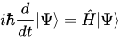
The tally of quantum numbers varies from system to system and has no universal answer. Hence these parameters must be found for each system to be analyzed. A quantized system requires at least one quantum number. The dynamics (i.e. time evolution) of any quantum system are described by a quantum operator in the form of a Hamiltonian, H. There is one quantum number of the system corresponding to the system's energy; i.e., one of the eigenvalues of the Hamiltonian. There is also one quantum number for each linearly independent operator O that commutes with the Hamiltonian. A complete set of commuting observables (CSCO) that commute with the Hamiltonian characterizes the system with all its quantum numbers. There is a one-to-one relationship between the quantum numbers and the operators of the CSCO, with each quantum number taking one of the eigenvalues of its corresponding operator. As a result of the different basis that may be arbitrarily chosen to form a complete set of commuting operators, different sets of quantum numbers may be used for the description of the same system in different situations.

Four quantum numbers can describe an electron energy level in a hydrogen-like atom completely:

• Principal quantum number (n)
• Azimuthal quantum number (ℓ)
• Magnetic quantum number (m_ℓ)
• Spin quantum number (m_s)

These quantum numbers are also used in the classical description of nuclear particle states (e.g. protons and neutrons).^{[citation needed]} A quantum description of molecular orbitals requires other quantum numbers, because the symmetries of the molecular system are different.

The principal quantum number describes the electron shell of an electron. The value of n ranges from 1 to the shell containing the outermost electron of that atom, that is^[12] $${\displaystyle n=1,2,\ldots }$$

For example, in caesium (Cs), the outermost valence electron is in the shell with energy level 6, so an electron in caesium can have an n value from 1 to 6. The average distance between the electron and the nucleus increases with n.

The azimuthal quantum number, also known as the orbital angular momentum quantum number, describes the subshell, and gives the magnitude of the orbital angular momentum through the relation $${\displaystyle L^{2}=\hbar ^{2}\ell (\ell +1).}$$

In chemistry and spectroscopy, ℓ = 0 is called s orbital, ℓ = 1, p orbital, ℓ = 2, d orbital, and ℓ = 3, f orbital.

The value of ℓ ranges from 0 to n − 1, so the first p orbital (ℓ = 1) appears in the second electron shell (n = 2), the first d orbital (ℓ = 2) appears in the third shell (n = 3), and so on:^[13] $${\displaystyle \ell =0,1,2,\ldots ,n-1}$$

A quantum number beginning in n = 3, ℓ = 0, describes an electron in the s orbital of the third electron shell of an atom. In chemistry, this quantum number is very important, since it specifies the shape of an atomic orbital and strongly influences chemical bonds and bond angles. The azimuthal quantum number can also denote the number of angular nodes present in an orbital. For example, for p orbitals, ℓ = 1 and thus the amount of angular nodes in a p orbital is 1.

The magnetic quantum number describes the specific orbital within the subshell, and yields the projection of the orbital angular momentum along a specified axis: $${\displaystyle L_{z}=m_{\ell }\hbar }$$

The values of m_ℓ range from −ℓ to ℓ, with integer intervals.^{[14][page needed]}

The s subshell (ℓ = 0) contains only one orbital, and therefore the m_ℓ of an electron in an s orbital will always be 0. The p subshell (ℓ = 1) contains three orbitals, so the m_ℓ of an electron in a p orbital will be −1, 0, or 1. The d subshell (ℓ = 2) contains five orbitals, with m_ℓ values of −2, −1, 0, 1, and 2.

The spin magnetic quantum number describes the intrinsic spin angular momentum of the electron within each orbital and gives the projection of the spin angular momentum S along the specified axis: $${\displaystyle S_{z}=m_{s}\hbar }$$

In general, the values of m_s range from −s to s, where s is the spin quantum number, associated with the magnitude of particle's intrinsic spin angular momentum:^[15] $${\displaystyle m_{s}=-s,-s+1,-s+2,\cdots ,s-2,s-1,s}$$

An electron state has spin number s = ⁠1/2⁠, consequently m_s will be +⁠1/2⁠ ("spin up") or −⁠1/2⁠ "spin down" states. Since electron are fermions they obey the Pauli exclusion principle: each electron state must have different quantum numbers. Therefore, every orbital will be occupied with at most two electrons, one for each spin state.

A multi-electron atom can be modeled qualitatively as a hydrogen like atom with higher nuclear charge and correspondingly more electrons. The occupation of the electron states in such an atom can be predicted by the Aufbau principle and Hund's empirical rules for the quantum numbers. The Aufbau principle fills orbitals based on their principal and azimuthal quantum numbers (lowest n + ℓ first, with lowest n breaking ties; Hund's rule favors unpaired electrons in the outermost orbital). These rules are empirical but they can be related to electron physics.^{[16]: 10 [17]: 260}

When one takes the spin–orbit interaction into consideration, the L and S operators no longer commute with the Hamiltonian, and the eigenstates of the system no longer have well-defined orbital angular momentum and spin. Thus another set of quantum numbers should be used. This set includes^[18][19]

1. The total angular momentum quantum number: $${\displaystyle j=|\ell \pm s|,}$$ which gives the total angular momentum through the relation $${\displaystyle J^{2}=\hbar ^{2}j(j+1).}$$
2. The projection of the total angular momentum along a specified axis: $${\displaystyle m_{j}=-j,-j+1,-j+2,\cdots ,j-2,j-1,j}$$ analogous to the above and satisfies both $${\displaystyle m_{j}=m_{\ell }+m_{s},}$$ and $${\displaystyle |m_{\ell }+m_{s}|\leq j.}$$
3. Parity
   This is the eigenvalue under reflection: positive (+1) for states which came from even ℓ and negative (−1) for states which came from odd ℓ. The former is also known as even parity and the latter as odd parity, and is given by$${\displaystyle P=(-1)^{\ell }.}$$

For example, consider the following 8 states, defined by their quantum numbers:

	n	ℓ	mℓ	ms		ℓ + s	ℓ − s	mℓ + ms
(1)	2	1	1	+⁠1/2⁠		⁠3/2⁠	⁠1/2⁠	⁠3/2⁠
(2)	2	1	1	−⁠1/2⁠		⁠3/2⁠	⁠1/2⁠	⁠1/2⁠
(3)	2	1	0	+⁠1/2⁠		⁠3/2⁠	⁠1/2⁠	⁠1/2⁠
(4)	2	1	0	−⁠1/2⁠		⁠3/2⁠	⁠1/2⁠	−⁠1/2⁠
(5)	2	1	−1	+⁠1/2⁠		⁠3/2⁠	⁠1/2⁠	−⁠1/2⁠
(6)	2	1	−1	−⁠1/2⁠		⁠3/2⁠	⁠1/2⁠	−⁠3/2⁠
(7)	2	0	0	+⁠1/2⁠		⁠1/2⁠	−⁠1/2⁠	⁠1/2⁠
(8)	2	0	0	−⁠1/2⁠		⁠1/2⁠	−⁠1/2⁠	−⁠1/2⁠

The quantum states in the system can be described as linear combination of these 8 states. However, in the presence of spin–orbit interaction, if one wants to describe the same system by 8 states that are eigenvectors of the Hamiltonian (i.e. each represents a state that does not mix with others over time), we should consider the following 8 states:

j	mj	parity
⁠3/2⁠	⁠3/2⁠	odd	coming from state (1) above
⁠3/2⁠	⁠1/2⁠	odd	coming from states (2) and (3) above
⁠3/2⁠	−⁠1/2⁠	odd	coming from states (4) and (5) above
⁠3/2⁠	−⁠3/2⁠	odd	coming from state (6) above
⁠1/2⁠	⁠1/2⁠	odd	coming from states (2) and (3) above
⁠1/2⁠	−⁠1/2⁠	odd	coming from states (4) and (5) above
⁠1/2⁠	⁠1/2⁠	even	coming from state (7) above
⁠1/2⁠	−⁠1/2⁠	even	coming from state (8) above

In nuclei, the entire assembly of protons and neutrons (nucleons) has a resultant angular momentum due to the angular momenta of each nucleon, usually denoted I. If the total angular momentum of a neutron is j_n = ℓ + s and for a proton is j_p = ℓ + s (where s for protons and neutrons happens to be ⁠1/2⁠ again (see note)), then the nuclear angular momentum quantum numbers I are given by: $${\displaystyle I=|j_{n}-j_{p}|,|j_{n}-j_{p}|+1,|j_{n}-j_{p}|+2,\cdots ,(j_{n}+j_{p})-2,(j_{n}+j_{p})-1,(j_{n}+j_{p})}$$ Note: The orbital angular momenta of the nuclear (and atomic) states are all integer multiples of ħ while the intrinsic angular momentum of the neutron and proton are half-integer multiples. It should be immediately apparent that the combination of the intrinsic spins of the nucleons with their orbital motion will always give half-integer values for the total spin, I, of any odd-A nucleus and integer values for any even-A nucleus.

Parity with the number I is used to label nuclear angular momentum states, examples for some isotopes of hydrogen (H), carbon (C), and sodium (Na) are;^[20]

1 1H	I = (⁠1/2⁠)+		9 6C	I = (⁠3/2⁠)−		20 11Na	I = 2+
2 1H	I = 1+		10 6C	I = 0+		21 11Na	I = (⁠3/2⁠)+
3 1H	I = (⁠1/2⁠)+		11 6C	I = (⁠3/2⁠)−		22 11Na	I = 3+
			12 6C	I = 0+		23 11Na	I = (⁠3/2⁠)+
			13 6C	I = (⁠1/2⁠)−		24 11Na	I = 4+
			14 6C	I = 0+		25 11Na	I = (⁠5/2⁠)+
			15 6C	I = (⁠1/2⁠)+		26 11Na	I = 3+

The reason for the unusual fluctuations in I, even by differences of just one nucleon, are due to the odd and even numbers of protons and neutrons – pairs of nucleons have a total angular momentum of zero (just like electrons in orbitals), leaving an odd or even number of unpaired nucleons. The property of nuclear spin is an important factor for the operation of NMR spectroscopy in organic chemistry,^[19] and MRI in nuclear medicine,^[20] due to the nuclear magnetic moment interacting with an external magnetic field.

Elementary particles contain many quantum numbers which are usually said to be intrinsic to them. However, the elementary particles are quantum states of the Standard Model of particle physics, and hence the quantum numbers of these particles bear the same relation to the Hamiltonian of this model as the quantum numbers of the Bohr atom does to its Hamiltonian. In other words, each quantum number denotes a symmetry of the problem. It is more useful in quantum field theory to distinguish between spacetime and internal symmetries.

Typical quantum numbers related to spacetime symmetries are spin (related to rotational symmetry), the parity, C-parity and T-parity (related to the Poincaré symmetry of spacetime). Typical internal symmetries^{[clarification needed]} are lepton number and baryon number or the electric charge. (For a full list of quantum numbers of this kind see the article on flavour.)

Most conserved quantum numbers are additive, so in an elementary particle reaction, the sum of the quantum numbers should be the same before and after the reaction. However, some, usually called parities, are multiplicative; i.e., their product is conserved. All multiplicative quantum numbers belong to a symmetry (like parity) in which applying the symmetry transformation twice is equivalent to doing nothing (involution).

• Electron configuration