Hubbry Logo
search
logo
2216201

Electrostatics

logo
Community Hub0 Subscribers
Read side by side
from Wikipedia
A tabby cat covered in packing peanuts.
Foam peanuts clinging to a cat's fur due to static electricity. The cat's fur becomes charged due to the triboelectric effect. The electric field of the charged fur causes polarization of the molecules of the foam due to electrostatic induction, resulting in a slight attraction of the light plastic pieces to the fur.[1][2][3][4] This effect is also the cause of static cling in clothes.

Electrostatics is a branch of physics that studies slow-moving or stationary electric charges on macroscopic objects where quantum effects can be neglected. Under these circumstances the electric field, electric potential, and the charge density are related without complications from magnetic effects.

Since classical antiquity, it has been known that some materials, such as amber, attract lightweight particles after rubbing.[citation needed] The Greek word ḗlektron (ἤλεκτρον), meaning 'amber', was thus the root of the word electricity. Electrostatic phenomena arise from the forces that electric charges exert on each other. Such forces are described by Coulomb's law.

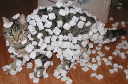
There are many examples of electrostatic phenomena, from those as simple as the attraction of plastic wrap to one's hand after it is removed from a package, to the apparently spontaneous explosion of grain silos, the damage of electronic components during manufacturing, and photocopier and laser printer operation.

Coulomb's law

[edit]

Coulomb's law states that:[5]

The magnitude of the electrostatic force of attraction or repulsion between two point charges is directly proportional to the product of the magnitudes of charges and inversely proportional to the square of the distance between them.

The force is along the straight line joining them. If the two charges have the same sign, the electrostatic force between them is repulsive; if they have different signs, the force between them is attractive.

If is the distance (in meters) between two charges, then the force between two point charges and is:

where ε0 = 8.8541878188(14)×10−12 F⋅m−1[6] is the vacuum permittivity.[7]

The SI unit of ε0 is equivalently A2s4 ⋅kg−1⋅m−3 or C2N−1⋅m−2 or F⋅m−1.

Electric field

[edit]
The electrostatic field (lines with arrows) of a nearby positive charge (+) causes the mobile charges in conductive objects to separate due to electrostatic induction. Negative charges (blue) are attracted and move to the surface of the object facing the external charge. Positive charges (red) are repelled and move to the surface facing away. These induced surface charges are exactly the right size and shape so their opposing electric field cancels the electric field of the external charge throughout the interior of the metal. Therefore, the electrostatic field everywhere inside a conductive object is zero, and the electrostatic potential is constant.

The electric field, , in units of newtons per coulomb or volts per meter, is a vector field that can be defined everywhere, except at the location of point charges (where it diverges to infinity).[8] It is defined as the electrostatic force on a hypothetical small test charge at the point due to Coulomb's law, divided by the charge

Electric field lines are useful for visualizing the electric field. Field lines begin on positive charge and terminate on negative charge. They are parallel to the direction of the electric field at each point, and the density of these field lines is a measure of the magnitude of the electric field at any given point.

A collection of particles of charge , located at points (called source points) generates the electric field at (called the field point) of:[8]

where is the displacement vector from a source point to the field point , and is the unit vector of the displacement vector that indicates the direction of the field due to the source at point . For a single point charge, , at the origin, the magnitude of this electric field is and points away from that charge if it is positive. The fact that the force (and hence the field) can be calculated by summing over all the contributions due to individual source particles is an example of the superposition principle. The electric field produced by a distribution of charges is given by the volume charge density and can be obtained by converting this sum into a triple integral:

Gauss's law

[edit]

Gauss's law[9][10] states that "the total electric flux through any closed surface in free space of any shape drawn in an electric field is proportional to the total electric charge enclosed by the surface." Many numerical problems can be solved by considering a Gaussian surface around a body. Mathematically, Gauss's law takes the form of an integral equation:

where is a volume element. If the charge is distributed over a surface or along a line, replace by or . The divergence theorem allows Gauss's law to be written in differential form:

where is the divergence operator.

Poisson and Laplace equations

[edit]

The definition of electrostatic potential, combined with the differential form of Gauss's law (above), provides a relationship between the potential Φ and the charge density ρ:

This relationship is a form of Poisson's equation.[11] In the absence of unpaired electric charge, the equation becomes Laplace's equation:

Electrostatic approximation

[edit]
Summary of electrostatic relations between electric potential, electric field and charge density. Here, .

If the electric field in a system can be assumed to result from static charges, that is, a system that exhibits no significant time-varying magnetic fields, the system is justifiably analyzed using only the principles of electrostatics. This is called the "electrostatic approximation".[12]

The validity of the electrostatic approximation rests on the assumption that the electric field is irrotational, or nearly so:

From Faraday's law, this assumption implies the absence or near-absence of time-varying magnetic fields:

In other words, electrostatics does not require the absence of magnetic fields or electric currents. Rather, if magnetic fields or electric currents do exist, they must not change with time, or in the worst-case, they must change with time only very slowly. In some problems, both electrostatics and magnetostatics may be required for accurate predictions, but the coupling between the two can still be ignored. Electrostatics and magnetostatics can both be seen as non-relativistic Galilean limits for electromagnetism.[13] In addition, conventional electrostatics ignore quantum effects which have to be added for a complete description.[8]: 2 

Electrostatic potential

[edit]

As the electric field is irrotational, it is possible to express the electric field as the gradient of a scalar function, , called the electrostatic potential (also known as the voltage). An electric field, , points from regions of high electric potential to regions of low electric potential, expressed mathematically as

The gradient theorem can be used to establish that the electrostatic potential is the amount of work per unit charge required to move a charge from point to point with the following line integral:

From these equations, we see that the electric potential is constant in any region for which the electric field vanishes (such as occurs inside a conducting object).

Electrostatic energy

[edit]

A test particle's potential energy, , can be calculated from a line integral of the work, . We integrate from a point at infinity, and assume a collection of particles of charge , are already situated at the points . This potential energy (in Joules) is:

where is the distance of each charge from the test charge , which situated at the point , and is the electric potential that would be at if the test charge were not present. If only two charges are present, the potential energy is . The total electric potential energy due a collection of N charges is calculating by assembling these particles one at a time:

where the following sum from, j = 1 to N, excludes i = j:

This electric potential, is what would be measured at if the charge were missing. This formula obviously excludes the (infinite) energy that would be required to assemble each point charge from a disperse cloud of charge. The sum over charges can be converted into an integral over charge density using the prescription :

This second expression for electrostatic energy uses the fact that the electric field is the negative gradient of the electric potential, as well as vector calculus identities in a way that resembles integration by parts. These two integrals for electric field energy seem to indicate two mutually exclusive formulas for electrostatic energy density, namely and ; they yield equal values for the total electrostatic energy only if both are integrated over all space.

Electrostatic pressure

[edit]

Inside of an electrical conductor, there is no electric field.[14] The external electric field has been balanced by surface charges due to movement of charge carriers, either to or from other parts of the material, known as electrostatic induction. The equation connecting the field just above a small patch of the surface and the surface charge is where

  • = the surface unit normal vector,
  • = the surface charge density.

The average electric field, half the external value,[15] also exerts a force (Coulomb's law) on the conductor patch where the force is given by

.

In terms of the field just outside the surface, the force is equivalent to a pressure given by:

This pressure acts normal to the surface of the conductor, independent of whether: the mobile charges are electrons, holes or mobile protons; the sign of the surface charge; or the sign of the surface normal component of the electric field.[15] Note that there is a similar form for electrostriction in a dielectric.[16]

See also

[edit]

References

[edit]

Further reading

[edit]
[edit]
Revisions and contributorsEdit on WikipediaRead on Wikipedia
from Grokipedia
Electrostatics is the branch of physics that deals with electric charges at rest and the stationary electric fields they produce, encompassing the study of forces between charged particles in equilibrium.[1] It focuses on the properties of electrical forces arising from charge distributions, where charges do not move relative to the objects they reside in, as exemplified by phenomena like static electricity.[2] The foundational principle is Coulomb's law, which quantifies the electrostatic force between two point charges as directly proportional to the product of their charge magnitudes and inversely proportional to the square of the separation distance between them, following an inverse-square relationship analogous to gravity but much stronger at short ranges.[3] Electric charge, the source of these forces, is a fundamental property of matter quantized in discrete units, with the elementary charge of an electron or proton being approximately 1.602×10191.602 \times 10^{-19} coulombs (C), and it obeys the law of conservation, meaning the total charge in an isolated system remains constant.[4] Key concepts include the electric field, a vector field surrounding charges that exerts forces on other charges within it, defined such that the force on a test charge qq is F=qE\mathbf{F} = q\mathbf{E}, where E\mathbf{E} is independent of the test charge.[3] This leads to tools like Gauss's law, which relates the electric flux through a closed surface to the enclosed charge, enabling calculations for symmetric charge distributions: EdA=Qencϵ0\oint \mathbf{E} \cdot d\mathbf{A} = \frac{Q_{\text{enc}}}{\epsilon_0}, with ϵ0\epsilon_0 as the vacuum permittivity.[5] Electrostatics also involves electric potential, the scalar potential energy per unit charge, from which the electric field derives as the negative gradient, E=V\mathbf{E} = -\nabla V, facilitating energy-based analyses of charge configurations like capacitors, which store energy in the form U=12CV2U = \frac{1}{2}CV^2.[5] The field is conservative, meaning the work done by the electric force around a closed path is zero, and the principle of superposition applies, allowing complex systems to be analyzed by summing contributions from individual charges.[3] Historically, observations of static electricity date back to ancient times, with systematic study beginning in the 18th century through experiments by figures like Charles-Augustin de Coulomb, who quantified the force law using a torsion balance.[4] In modern contexts, electrostatics underpins diverse applications, including Van de Graaff generators for high-voltage research, xerography in photocopiers and laser printers via charged toner particles, electrostatic painting for uniform coating, and electrostatic precipitators that remove over 99% of particulate matter from industrial exhaust gases.[6] These principles extend to natural phenomena like lightning and atmospheric electricity, highlighting electrostatics' role in both fundamental science and technology.[6]

Fundamental Concepts

Electric Charge

Electric charge is a fundamental physical property of matter that causes it to experience a force within an electromagnetic field. It manifests in two distinct types: positive charge, primarily associated with protons, and negative charge, carried by electrons. Like charges repel one another, while opposite charges attract, forming the basis of electrostatic interactions.[7][8][9] The modern convention of labeling charges as positive and negative originated with Benjamin Franklin's experiments in the mid-1750s, where he distinguished the two forms based on their behaviors in frictional electricity and lightning. In 1909, Robert Millikan conducted the oil-drop experiment, which demonstrated that electric charge is quantized, occurring only in discrete multiples of the elementary charge e=1.602176634×10¹⁹e = 1.602176634 \times 10^{-19} C.[10][11][12] The law of conservation of electric charge states that the total electric charge in an isolated system remains constant, as charge cannot be created or destroyed, only transferred. This principle is exemplified in triboelectric charging, where friction between materials leads to electron transfer; for instance, rubbing a glass rod with silk causes the glass to gain a positive charge while the silk becomes negative, following their positions in the triboelectric series.[13] The international unit of electric charge is the coulomb (C), defined as the quantity of charge transported by a constant current of one ampere over one second. Early measurements of charge relied on electrometers, devices that detect and quantify charge through the mechanical deflection produced by electrostatic repulsion between similarly charged leaves or needles.[14][15][16]

Coulomb's Law

Coulomb's law quantifies the electrostatic force between two stationary point charges q1q_1 and q2q_2 separated by a distance rr in vacuum. The force F\vec{F} is given by
F=kq1q2r2r^, \vec{F} = k \frac{q_1 q_2}{r^2} \hat{r},
where k=14πϵ0k = \frac{1}{4\pi\epsilon_0} is Coulomb's constant, ϵ0=8.85×10¹²C2/Nm2\epsilon_0 = 8.85 \times 10^{-12} \, \mathrm{C^2/N \cdot m^2} is the vacuum permittivity, and r^\hat{r} is the unit vector pointing from q1q_1 to q2q_2.[17][5] This vector form indicates that the force is central, acting along the line joining the charges, and its magnitude is F=kq1q2r2F = k \frac{|q_1 q_2|}{r^2}.[18] The law was empirically established through experiments by Charles-Augustin de Coulomb in 1785 using a torsion balance, an instrument he designed to measure the torsional deflection caused by repulsive or attractive forces between charged spheres.[19][20] In these experiments, Coulomb suspended one charged object on a fine wire and observed the equilibrium twist when interacting with another fixed charge, confirming the inverse-square dependence of the force on distance and its proportionality to the product of the charges.[21] The direction of the force follows from the sign of q1q2q_1 q_2: if the charges have the same sign (both positive or both negative), the force is repulsive, directed away from each other along r^\hat{r} or r^-\hat{r}; if opposite signs, it is attractive, pulling them together.[5] This arises directly from the positive value of [k](/page/K)[k](/page/K) and the scalar product q1q2q_1 q_2, yielding a positive force magnitude that aligns with repulsion for like charges and requires reversing the direction vector for attraction in the two-charge system.[18] Coulomb's law strictly applies to point charges at rest in vacuum, where velocities are negligible and no magnetic effects arise; it assumes non-relativistic conditions and neglects medium polarization effects present in dielectrics.[5] For continuous charge distributions, such as lines, surfaces, or volumes, the law extends by integrating over infinitesimal charge elements: the total force on a test charge is F=kqρ(r)(rr)rr3dV\vec{F} = k q \int \frac{\rho(\vec{r}') (\vec{r} - \vec{r}')}{|\vec{r} - \vec{r}'|^3} dV', where ρ\rho is the charge density, though explicit computation requires specific geometries.[18] This inverse-square form mirrors Newton's law of universal gravitation, $ \vec{F} = -G \frac{m_1 m_2}{r^2} \hat{r} $, where GG is the gravitational constant, highlighting a structural similarity in the central, distance-dependent forces between interacting pairs, though electrostatic forces are vastly stronger and can be attractive or repulsive depending on charge signs.

Electric Field

Definition and Properties

The electric field E\vec{E} is a vector field that describes the electric force experienced per unit positive test charge at any point in space. It is formally defined as the limit of the ratio of the electrostatic force F\vec{F} on a small positive test charge q0q_0 to the magnitude of that charge, as q0q_0 approaches zero to avoid perturbing the source configuration:
E=limq00Fq0. \vec{E} = \lim_{q_0 \to 0} \frac{\vec{F}}{q_0}.
This definition captures the force that would act on any positive charge placed at the location, independent of the specific test charge used.[22][23] For a single point charge qq located at the origin, the electric field at a distance rr along the radial direction is given by
E=14πϵ0qr2r^, \vec{E} = \frac{1}{4\pi\epsilon_0} \frac{q}{r^2} \hat{r},
where ϵ0\epsilon_0 is the vacuum permittivity, and r^\hat{r} is the unit vector pointing away from the charge. This expression arises directly from Coulomb's law by considering the force on a test charge at distance rr. The field points radially outward from a positive charge and inward toward a negative charge, with magnitude decreasing as the inverse square of the distance.[22][23] Key properties of the electrostatic field include its vector nature, which means it has both magnitude and direction at every point; its additivity via the superposition principle, where the total field from multiple charges is the vector sum of individual fields; its conservative character in electrostatic equilibrium, expressed mathematically as ×E=0\nabla \times \vec{E} = 0, implying that the work done by the field around any closed path is zero; and its inverse-square decay for point sources, reflecting the underlying pairwise nature of electrostatic interactions. The SI units of the electric field are newtons per coulomb (N/C), equivalently volts per meter (V/m).[22][23][24] Electric field lines provide a visual representation of the field's direction and relative strength. These imaginary lines are drawn such that their direction at any point is tangent to the field vector there, originating from positive charges (or at infinity) and terminating on negative charges (or at infinity). The density of the lines in a region is proportional to the magnitude of the field strength, with closer spacing indicating stronger fields. Visualization techniques, such as aligning small particles like grass seeds in oil under an applied field or computational simulations, analogously reveal patterns similar to iron filings tracing magnetic fields.[25][23]

Gauss's Law

Gauss's law is a fundamental principle in electrostatics that relates the electric flux through a closed surface to the total electric charge enclosed within that surface. It is expressed mathematically as
SEdA=Qencϵ0, \oint_S \vec{E} \cdot d\vec{A} = \frac{Q_{\mathrm{enc}}}{\epsilon_0},
where E\vec{E} is the electric field, dAd\vec{A} is the differential area vector on the closed surface SS, QencQ_{\mathrm{enc}} is the net charge enclosed by SS, and ϵ0\epsilon_0 is the vacuum permittivity.[26] This integral form highlights the law's reliance on symmetry, making it particularly useful for calculating electric fields in situations with high geometric symmetry, rather than directly integrating Coulomb's law for complex charge distributions.[27] The law can be derived from Coulomb's law by considering the flux due to a point charge. For a point charge qq at the origin, the electric field is radial, and the flux through a closed surface is computed using solid-angle arguments: the total solid angle subtended by any closed surface enclosing the charge is 4π4\pi steradians, leading to EdA=qϵ0\oint \vec{E} \cdot d\vec{A} = \frac{q}{\epsilon_0}. Extending this to arbitrary charge distributions via superposition yields the general form, as the contributions from each infinitesimal charge element dqdq sum to the enclosed charge. Alternatively, applying the divergence theorem to the field expression from Coulomb's law transforms the integral into a volume integral of the divergence, confirming the result.[5][28] In its differential form, Gauss's law is E=ρϵ0\nabla \cdot \vec{E} = \frac{\rho}{\epsilon_0}, where ρ\rho is the charge density; this local relation is obtained by applying the divergence theorem to the integral form over an infinitesimal volume.[29] This version connects electrostatics to the broader framework of partial differential equations and is one of Maxwell's equations, which unify electricity, magnetism, and optics.[30] Gauss's law excels in applications involving symmetric charge distributions, where the field magnitude is constant over the Gaussian surface. For an infinite plane with surface charge density σ\sigma, a cylindrical Gaussian surface perpendicular to the plane yields E=σ2ϵ0E = \frac{\sigma}{2\epsilon_0}, independent of distance. For an infinite line charge with linear density λ\lambda, a cylindrical surface gives E=λ2πϵ0rE = \frac{\lambda}{2\pi \epsilon_0 r}. For a uniformly charged spherical shell of radius RR and total charge QQ, the field is zero inside (r<Rr < R) and E=Q4πϵ0r2E = \frac{Q}{4\pi \epsilon_0 r^2} outside (r>Rr > R).[26][27] The law is named after Carl Friedrich Gauss, who rediscovered and formalized it in 1835 in the context of inverse-square forces, building on earlier work by Joseph-Louis Lagrange in 1773; it forms the cornerstone of electrostatic theory as part of Maxwell's equations.[31]

Superposition and Field Lines

The superposition principle in electrostatics states that the total electric field at any point due to multiple charges is the vector sum of the electric fields produced by each charge individually.[5] This principle arises from the linearity of Coulomb's law, which describes the force between two point charges as proportional to the product of their charges and inversely proportional to the square of their separation distance, allowing forces (and thus fields) to add linearly without interference.[32] Furthermore, the electrostatic limit of Maxwell's equations—specifically, E=ρ/ϵ0\nabla \cdot \vec{E} = \rho / \epsilon_0 and ×E=0\nabla \times \vec{E} = 0—is linear in the fields and charge density, ensuring that solutions superpose for arbitrary charge distributions.[33] For example, consider two point charges: the electric field at a point equidistant from equal positive charges points away from both along the perpendicular bisector, resulting in a net field twice the magnitude of one charge's contribution in that direction. In the case of an electric dipole—two equal and opposite charges separated by a small distance—the fields near the charges are complex, but far from the dipole (at distances much larger than the separation), the opposing contributions partially cancel, yielding a net field that falls off as 1/r31/r^3 and aligns with the dipole axis.[34] This approximation simplifies analysis of neutral systems like molecules, where the dipole moment p=qd\vec{p} = q \vec{d} (with qq the charge magnitude and d\vec{d} the displacement vector) dominates the far-field behavior.[35] Electric field lines provide a visual representation of the electric field's direction and relative strength, defined as imaginary lines tangent to the field vector at every point.[25] Key rules for drawing these lines include: they originate from positive charges (or extend to infinity for isolated positives) and terminate on negative charges (or from infinity for isolated negatives); they never cross, as the field has a unique direction at each point; the density of lines is proportional to field strength, with more lines indicating stronger fields; and lines are closer together in regions of higher field magnitude.[36] Qualitative sketches illustrate these for common configurations. For a single positive point charge (monopole), lines radiate symmetrically outward in all directions, becoming sparser with distance to reflect the 1/r21/r^2 field decay.[37] In a dipole, lines emerge from the positive charge, curve around to enter the negative charge, forming closed loops that bulge outward along the equatorial plane, with the tightest spacing midway between the charges where the field is strongest.[38] For a uniform field, such as between parallel oppositely charged plates, lines are straight, parallel, and equally spaced, indicating constant magnitude and direction.[39] Practically, the superposition principle enables prediction of field cancellation in neutral systems, such as atoms or molecules, where positive and negative charges balance to produce weak external fields, facilitating the study of induced dipoles in external fields.[5] It also allows qualitative predictions without full calculations, such as estimating field patterns in complex charge arrangements by mentally overlaying individual contributions.[40] However, field lines are merely illustrative tools for visualization and do not represent actual paths of charged particles, which follow parabolic trajectories under constant fields due to inertia.[36]

Electrostatic Potential

Definition and Gradient Relation

The electrostatic potential $ V $ at a position $ \vec{r} $ due to an electrostatic field is the amount of work done per unit positive test charge to bring it slowly from infinity to $ \vec{r} $, expressed through the line integral $ V(\vec{r}) = -\int_{\infty}^{\vec{r}} \vec{E} \cdot d\vec{l} $, where $ \vec{E} $ is the electric field and the integral is taken along any path from infinity to $ \vec{r} $.[41] This definition assumes the potential vanishes at infinity for localized charge distributions, a standard convention in electrostatics.[42] The electrostatic field $ \vec{E} $ is conservative, meaning the line integral is path-independent, as the work done by the field depends only on the endpoints and not the route taken.[43][44] For a single point charge $ q $ at the origin, the potential simplifies to $ V(r) = \frac{1}{4\pi\epsilon_0} \frac{q}{r} $, where $ r = |\vec{r}| $ is the distance from the charge and $ \epsilon_0 $ is the vacuum permittivity; this follows directly from integrating the Coulomb field along a radial path.[45][46] The relation between the potential and the electric field is given by $ \vec{E} = -\nabla V $, the negative gradient of the scalar potential, which in Cartesian coordinates yields the components $ E_x = -\frac{\partial V}{\partial x} $, $ E_y = -\frac{\partial V}{\partial y} $, and $ E_z = -\frac{\partial V}{\partial z} $.[47][48] This vector calculus relation highlights how the directional field $ \vec{E} $ derives from the scalar $ V $, facilitating computations in symmetric systems. Surfaces of constant potential, known as equipotential surfaces, are everywhere perpendicular to the electric field lines, since the tangential component of $ \vec{E} $ vanishes on such surfaces, implying no work is done moving a charge along them.[49][50] The unit of electric potential is the volt (V), defined such that 1 V = 1 J/C, representing the potential difference across which 1 C of charge experiences 1 J of work.[51] Voltmeters measure potential differences by connecting in parallel to the points of interest, drawing negligible current through a high internal resistance to approximate the open-circuit voltage without significantly perturbing the field.[52] Due to the linearity of electrostatics, the superposition principle applies to potentials as scalars: the total potential at any point from multiple charges is the algebraic sum of the individual potentials, simplifying calculations compared to vector addition for fields.[53][46]

Poisson's and Laplace's Equations

In electrostatics, Poisson's equation governs the scalar potential VV in the presence of a charge density distribution ρ\rho. It is derived by combining Gauss's law in differential form, E=ρϵ0\nabla \cdot \vec{E} = \frac{\rho}{\epsilon_0}, with the relation between the electric field and potential, E=V\vec{E} = -\nabla V. Substituting yields (V)=ρϵ0\nabla \cdot (-\nabla V) = \frac{\rho}{\epsilon_0}, or equivalently,
2V=ρϵ0, \nabla^2 V = -\frac{\rho}{\epsilon_0},
where 2\nabla^2 is the Laplacian operator and ϵ0\epsilon_0 is the vacuum permittivity.[54] This second-order partial differential equation describes how the potential varies spatially due to localized charges. In regions devoid of charge, where ρ=0\rho = 0, the equation simplifies to Laplace's equation,
2V=0. \nabla^2 V = 0.
Laplace's equation arises naturally in charge-free spaces, such as between conductors or outside charge distributions, and its solutions represent harmonic functions that model equilibrium potentials.[54] The Laplacian operator 2\nabla^2 takes different explicit forms depending on the coordinate system, which is essential for solving these equations in problems with specific symmetries. In Cartesian coordinates (x,y,z)(x, y, z), it is
2V=2Vx2+2Vy2+2Vz2. \nabla^2 V = \frac{\partial^2 V}{\partial x^2} + \frac{\partial^2 V}{\partial y^2} + \frac{\partial^2 V}{\partial z^2}.
This form is straightforward for rectangular geometries but less convenient for cylindrical or spherical symmetries common in electrostatic problems. In spherical coordinates (r,θ,ϕ)(r, \theta, \phi), where rr is the radial distance, θ\theta the polar angle, and ϕ\phi the azimuthal angle, Laplace's equation becomes
1r2r(r2Vr)+1r2sinθθ(sinθVθ)+1r2sin2θ2Vϕ2=0. \frac{1}{r^2} \frac{\partial}{\partial r} \left( r^2 \frac{\partial V}{\partial r} \right) + \frac{1}{r^2 \sin \theta} \frac{\partial}{\partial \theta} \left( \sin \theta \frac{\partial V}{\partial \theta} \right) + \frac{1}{r^2 \sin^2 \theta} \frac{\partial^2 V}{\partial \phi^2} = 0.
Poisson's equation in spherical coordinates follows the same left-hand side equal to ρ/ϵ0-\rho / \epsilon_0. This form facilitates solutions for problems like point charges or spherical conductors using separation of variables.[55] For cylindrical coordinates (ρ,ϕ,z)(\rho, \phi, z), with ρ\rho the radial distance from the axis, ϕ\phi the azimuthal angle, and zz along the axis, the equation is
1ρρ(ρVρ)+1ρ22Vϕ2+2Vz2=0 \frac{1}{\rho} \frac{\partial}{\partial \rho} \left( \rho \frac{\partial V}{\partial \rho} \right) + \frac{1}{\rho^2} \frac{\partial^2 V}{\partial \phi^2} + \frac{\partial^2 V}{\partial z^2} = 0
for Laplace's case, and similarly for Poisson's with the right-hand side ρ/ϵ0-\rho / \epsilon_0. This is particularly useful for infinite line charges or coaxial geometries.[56] Solutions to these equations require appropriate boundary conditions to ensure physical relevance. The potential VV is continuous across interfaces, such as between dielectrics or at conductor surfaces. The normal component of the electric field, V/n-\partial V / \partial n, exhibits a discontinuity at surfaces with surface charge density σ\sigma, jumping by σ/ϵ0\sigma / \epsilon_0. For conductors, VV is constant on the surface, and the tangential field vanishes. At infinity, VV typically approaches zero for localized charges.[57] A key result is the uniqueness theorem, which guarantees that the solution to Poisson's or Laplace's equation in a given volume is uniquely determined by the charge distribution inside and the boundary values of VV (or its normal derivative) on the enclosing surface. To see this, suppose two solutions V1V_1 and V2V_2 satisfy the same equation and boundaries; their difference u=V1V2u = V_1 - V_2 obeys Laplace's equation with zero boundary values. Integrating (uu)=u2=0\nabla \cdot (u \nabla u) = |\nabla u|^2 = 0 over the volume and applying the divergence theorem yields u2dτ=0\int |\nabla u|^2 d\tau = 0, implying u=0\nabla u = 0 and thus u=u = constant, which is zero by boundaries. This theorem underpins computational methods and symmetry arguments in electrostatics.[57] Historically, Laplace's equation emerged in the late 1700s from Pierre-Simon Laplace's work on gravitational potentials in Mécanique Céleste, where he recognized that the Newtonian potential satisfies 2V=0\nabla^2 V = 0 in source-free regions around 1782. Poisson extended this in the 1810s, deriving the inhomogeneous form for electrostatics in memoirs on charge distributions, with the equation formalized in his 1823 paper on magnetism, 2V=4πkρ\nabla^2 V = -4\pi k \rho (in cgs units). These contributions laid the foundation for potential theory.[58][59]

Electrostatic Approximation and Phenomena

The electrostatic approximation is valid when electric charges are either at rest or moving with velocities much smaller than the speed of light, such that time-dependent magnetic fields and electromagnetic radiation effects can be neglected. Under this approximation, the electric field is irrotational (curl-free) and conservative, allowing the use of static equations like Coulomb's law and Gauss's law without considering retardation or inductive effects.[60] This framework enables the analysis of various electrostatic phenomena discussed below.

Energy and Capacitance

The electrostatic potential energy associated with a pair of point charges q1q_1 and q2q_2 separated by a distance rr is given by
U=14πϵ0q1q2r, U = \frac{1}{4\pi\epsilon_0} \frac{q_1 q_2}{r},
where ϵ0\epsilon_0 is the vacuum permittivity.[61] This expression represents the work required to assemble the charges from infinite separation, assuming they are stationary.[62] For a system of multiple point charges, the total potential energy is the sum over all unique pairs:
U=14πϵ0i<jqiqjrij. U = \frac{1}{4\pi\epsilon_0} \sum_{i < j} \frac{q_i q_j}{r_{ij}}.
This pairwise summation accounts for the interactions without double-counting.[62] For a continuous charge distribution with density ρ(r)\rho(\mathbf{r}), the electrostatic potential energy generalizes to the integral form
U=12ρ(r)V(r)dτ, U = \frac{1}{2} \int \rho(\mathbf{r}) V(\mathbf{r}) \, d\tau,
where V(r)V(\mathbf{r}) is the electric potential at position r\mathbf{r}, and the integral is over all space.[63] The factor of 1/21/2 arises from avoiding double-counting of interactions in the continuous limit, analogous to the discrete case.[62] This formulation connects the stored energy directly to the charge density and potential, providing a basis for analyzing complex configurations. An equivalent expression for the total energy can be derived in terms of the electric field E\mathbf{E}, revealing the energy density in the electrostatic field as
u=12ϵ0E2. u = \frac{1}{2} \epsilon_0 E^2.
The total energy is then the volume integral of this density:
U=12ϵ0E2dτ. U = \frac{1}{2} \epsilon_0 \int E^2 \, d\tau.
This field-based perspective highlights how energy is distributed throughout space, independent of the specific charge arrangement, and follows from vector calculus identities relating ρV\rho V to E\mathbf{E}.[62][63] Capacitors are devices designed to store electrostatic energy by maintaining separated charges on conductors. The capacitance CC of a capacitor is defined as the ratio of the magnitude of charge QQ on each conductor to the potential difference VV between them:
C=QV. C = \frac{Q}{V}.
The SI unit of capacitance is the farad (F), equivalent to one coulomb per volt.[64] A common example is the parallel-plate capacitor, consisting of two conducting plates of area AA separated by a small distance dd in vacuum, with capacitance
C=ϵ0Ad. C = \epsilon_0 \frac{A}{d}.
This formula assumes dAd \ll \sqrt{A} for uniform field approximation and neglects edge effects.[65] The energy stored in a capacitor follows from the work done to charge it and can be expressed as
U=12CV2=12Q2C. U = \frac{1}{2} C V^2 = \frac{1}{2} \frac{Q^2}{C}.
These equivalent forms derive from integrating the incremental work dU=VdqdU = V \, dq during charging, yielding a quadratic dependence on voltage or charge.[66] For the parallel-plate case, substituting the capacitance gives U=12ϵ0AdV2U = \frac{1}{2} \epsilon_0 \frac{A}{d} V^2, which matches the field energy integral with E=V/dE = V/d.[67] Introducing a dielectric material between the plates increases the capacitance by a factor κ>1\kappa > 1, known as the dielectric constant, without altering the charge or plate geometry.[64] This enhancement allows greater energy storage for the same voltage, as C=κCC' = \kappa C. The effect stems from the material's response to the field, though detailed mechanisms are beyond this scope. The Leyden jar, invented independently in 1745 by Ewald Jürgen von Kleist and Pieter van Musschenbroek, served as the first capacitor, consisting of a glass jar with conductive coatings inside and outside to store charge.[68] This device enabled early experiments in electrostatics by providing a means to accumulate and discharge electrical energy on demand.

Forces and Pressure on Conductors

In electrostatic equilibrium, a conductor exhibits zero electric field throughout its interior volume, with any excess charge residing exclusively on its surface. This configuration ensures that the entire conductor maintains a constant electrostatic potential, as free charges within the material redistribute to cancel any internal fields.[69] The mechanical force exerted on a conductor in an electrostatic field can be derived using the principle of virtual work, which relates the force to variations in the system's electrostatic energy UU. For a displacement along a coordinate xx, the force component is given by Fx=UxF_x = -\frac{\partial U}{\partial x} evaluated at constant charge QQ or constant potential VV, depending on the boundary conditions of the setup.[69][33] Just outside the surface of a conductor, the perpendicular component of the electric field EnE_n relates directly to the local surface charge density σ\sigma via Gauss's law applied to a Gaussian pillbox straddling the surface: σ=ϵ0En\sigma = \epsilon_0 E_n. This discontinuity in the field arises because the internal field is zero, confining the flux to the external side.[69] The electrostatic pressure on the conductor's surface, representing the outward force per unit area due to the repulsion of like charges, is derived by considering the force on a small surface element. This yields P=σ22ϵ0=12ϵ0En2P = \frac{\sigma^2}{2\epsilon_0} = \frac{1}{2} \epsilon_0 E_n^2, directed normal to the surface and away from the conductor.[70] A classic example is the attractive force between the oppositely charged plates of a parallel-plate capacitor. For plates of area AA separated by distance dd with total charge ±Q\pm Q, the uniform field between them is E=Q/(ϵ0A)E = Q/(\epsilon_0 A), leading to a force magnitude F=Q22ϵ0AF = \frac{Q^2}{2\epsilon_0 A} pulling the plates together, independent of dd for small separations where fringing is negligible.[71] For an isolated, uniformly charged spherical conductor, the net self-force is zero due to the symmetry of the charge distribution, which produces a radial field outside but no unbalanced tangential components to drive translation.[72] When a point charge qq is placed near an infinite grounded conducting plane, it induces an opposite surface charge distribution on the plane to maintain zero potential. The method of images models this by replacing the plane with a mirror image charge q-q at the symmetric position across the plane, allowing calculation of the field in the region of interest and the resulting force on qq as if interacting with the image.[73]

Dielectrics and Polarization

Dielectrics are insulating materials that do not conduct electricity freely but respond to an applied electric field by developing polarization, which alters the local electric field within the material.[74] This polarization arises from the displacement or reorientation of bound charges, such as electrons and ions, within the dielectric's atomic or molecular structure, leading to a net dipole moment per unit volume known as the polarization vector P\vec{P}.[75] The magnitude of P\vec{P} quantifies the extent of this alignment and is crucial for understanding how dielectrics modify electrostatic fields compared to vacuum. Polarization in dielectrics occurs through several mechanisms, each dominant in specific materials or conditions. Electronic polarization involves the distortion of electron clouds around atoms, shifting negative charge relative to the positive nucleus without permanent dipoles. Ionic polarization, prevalent in ionic crystals like NaCl, results from the relative displacement of oppositely charged ions in a lattice.[76] Orientational polarization occurs in materials with permanent molecular dipoles, such as water, where thermal motion randomizes dipoles in the absence of a field, but an applied field aligns them partially.[77] These processes collectively contribute to P\vec{P}, typically on the order of 10810^{-8} to 10610^{-6} C/m² in common dielectrics.[74] The presence of polarization introduces bound charges that affect the electric field. Volume bound charge density is given by ρb=P\rho_b = -\nabla \cdot \vec{P}, arising from spatial variations in polarization, while surface bound charge density is σb=Pn^\sigma_b = \vec{P} \cdot \hat{n}, where n^\hat{n} is the outward normal to the surface.[75] These bound charges oppose the applied field, reducing the net field inside the dielectric. To account for this, the electric displacement field D\vec{D} is defined as D=ϵ0E+P\vec{D} = \epsilon_0 \vec{E} + \vec{P}, where ϵ0\epsilon_0 is the vacuum permittivity and E\vec{E} is the electric field. In linear dielectrics, where polarization is proportional to the field, this simplifies to D=ϵ0ϵrE\vec{D} = \epsilon_0 \epsilon_r \vec{E}, with ϵr\epsilon_r the relative permittivity (dielectric constant).[78] Linear dielectrics are classified as isotropic if P\vec{P} is parallel to E\vec{E} with a scalar ϵr>1\epsilon_r > 1, or anisotropic if the response depends on direction, as in crystals, requiring a tensor description.[78] For example, water exhibits ϵr80\epsilon_r \approx 80 at room temperature due to strong orientational polarization from its polar molecules, while glass has ϵr510\epsilon_r \approx 5-10, primarily from electronic and ionic contributions.[79][80] This variation in ϵr\epsilon_r explains why dielectrics enhance capacitance and store more energy in electrostatic configurations. In the presence of dielectrics, Gauss's law is reformulated using D\vec{D} to focus on free charges: D=ρf\nabla \cdot \vec{D} = \rho_f, where ρf\rho_f denotes the density of free (unbound) charges.[81] This form simplifies calculations by excluding bound charges, which are incorporated into P\vec{P}. The energy stored in the electrostatic field within a dielectric is then U=12DEdτU = \frac{1}{2} \int \vec{D} \cdot \vec{E} \, d\tau, reflecting the work done to establish the field against the material's response.[82] For linear dielectrics, this reduces to 12ϵ0ϵrE2dτ\frac{1}{2} \epsilon_0 \epsilon_r \int E^2 \, d\tau, highlighting how higher ϵr\epsilon_r increases energy density.[83]

References

User Avatar
No comments yet.