Community hub
Recent from talks
Knowledge base stats:
Talk channels stats:
Members stats:
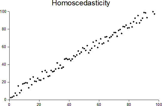
Homoscedasticity and heteroscedasticity
In statistics, a sequence of random variables is homoscedastic (/ˌhoʊmoʊskəˈdæstɪk/) if all its random variables have the same finite variance; this is also known as homogeneity of variance. The complementary notion is called heteroscedasticity, also known as heterogeneity of variance. The spellings homoskedasticity and heteroskedasticity are also frequently used. “Skedasticity” comes from the Ancient Greek word “skedánnymi”, meaning “to scatter”. Assuming a variable is homoscedastic when in reality it is heteroscedastic (/ˌhɛtəroʊskəˈdæstɪk/) results in unbiased but inefficient point estimates and in biased estimates of standard errors, and may result in overestimating the goodness of fit as measured by the Pearson coefficient.
The existence of heteroscedasticity is a major concern in regression analysis and the analysis of variance, as it invalidates statistical tests of significance that assume that the modelling errors all have the same variance. While the ordinary least squares (OLS) estimator is still unbiased in the presence of heteroscedasticity, it is inefficient and inference based on the assumption of homoskedasticity is misleading. In that case, generalized least squares (GLS) was frequently used in the past. Nowadays, standard practice in econometrics is to include Heteroskedasticity-consistent standard errors instead of using GLS, as GLS can exhibit strong bias in small samples if the actual skedastic function is unknown.
Because heteroscedasticity concerns expectations of the second moment of the errors, its presence is referred to as misspecification of the second order.
The econometrician Robert Engle was awarded the 2003 Nobel Memorial Prize for Economics for his studies on regression analysis in the presence of heteroscedasticity, which led to his formulation of the autoregressive conditional heteroscedasticity (ARCH) modeling technique.
Consider the linear regression equation where the dependent random variable equals the deterministic variable times coefficient plus a random disturbance term that has mean zero. The disturbances are homoscedastic if the variance of is a constant ; otherwise, they are heteroscedastic. In particular, the disturbances are heteroscedastic if the variance of depends on or on the value of . One way they might be heteroscedastic is if (an example of a scedastic function), so the variance is proportional to the value of .


More generally, if the variance-covariance matrix of disturbance across has a nonconstant diagonal, the disturbance is heteroscedastic. The matrices below are covariances when there are just three observations across time. The disturbance in matrix A is homoscedastic; this is the simple case where OLS is the best linear unbiased estimator. The disturbances in matrices B and C are heteroscedastic. In matrix B, the variance is time-varying, increasing steadily across time; in matrix C, the variance depends on the value of . The disturbance in matrix D is homoscedastic because the diagonal variances are constant, even though the off-diagonal covariances are non-zero and ordinary least squares is inefficient for a different reason: serial correlation.
Heteroscedasticity often occurs when there is a large difference among the sizes of the observations.
A classic example of heteroscedasticity is that of income versus expenditure on meals. A wealthy person may eat inexpensive food sometimes and expensive food at other times. A poor person will almost always eat inexpensive food. Therefore, people with higher incomes exhibit greater variability in expenditures on food.
Hub AI
Homoscedasticity and heteroscedasticity AI simulator
(@Homoscedasticity and heteroscedasticity_simulator)
Homoscedasticity and heteroscedasticity
In statistics, a sequence of random variables is homoscedastic (/ˌhoʊmoʊskəˈdæstɪk/) if all its random variables have the same finite variance; this is also known as homogeneity of variance. The complementary notion is called heteroscedasticity, also known as heterogeneity of variance. The spellings homoskedasticity and heteroskedasticity are also frequently used. “Skedasticity” comes from the Ancient Greek word “skedánnymi”, meaning “to scatter”. Assuming a variable is homoscedastic when in reality it is heteroscedastic (/ˌhɛtəroʊskəˈdæstɪk/) results in unbiased but inefficient point estimates and in biased estimates of standard errors, and may result in overestimating the goodness of fit as measured by the Pearson coefficient.
The existence of heteroscedasticity is a major concern in regression analysis and the analysis of variance, as it invalidates statistical tests of significance that assume that the modelling errors all have the same variance. While the ordinary least squares (OLS) estimator is still unbiased in the presence of heteroscedasticity, it is inefficient and inference based on the assumption of homoskedasticity is misleading. In that case, generalized least squares (GLS) was frequently used in the past. Nowadays, standard practice in econometrics is to include Heteroskedasticity-consistent standard errors instead of using GLS, as GLS can exhibit strong bias in small samples if the actual skedastic function is unknown.
Because heteroscedasticity concerns expectations of the second moment of the errors, its presence is referred to as misspecification of the second order.
The econometrician Robert Engle was awarded the 2003 Nobel Memorial Prize for Economics for his studies on regression analysis in the presence of heteroscedasticity, which led to his formulation of the autoregressive conditional heteroscedasticity (ARCH) modeling technique.
Consider the linear regression equation where the dependent random variable equals the deterministic variable times coefficient plus a random disturbance term that has mean zero. The disturbances are homoscedastic if the variance of is a constant ; otherwise, they are heteroscedastic. In particular, the disturbances are heteroscedastic if the variance of depends on or on the value of . One way they might be heteroscedastic is if (an example of a scedastic function), so the variance is proportional to the value of .
More generally, if the variance-covariance matrix of disturbance across has a nonconstant diagonal, the disturbance is heteroscedastic. The matrices below are covariances when there are just three observations across time. The disturbance in matrix A is homoscedastic; this is the simple case where OLS is the best linear unbiased estimator. The disturbances in matrices B and C are heteroscedastic. In matrix B, the variance is time-varying, increasing steadily across time; in matrix C, the variance depends on the value of . The disturbance in matrix D is homoscedastic because the diagonal variances are constant, even though the off-diagonal covariances are non-zero and ordinary least squares is inefficient for a different reason: serial correlation.
Heteroscedasticity often occurs when there is a large difference among the sizes of the observations.
A classic example of heteroscedasticity is that of income versus expenditure on meals. A wealthy person may eat inexpensive food sometimes and expensive food at other times. A poor person will almost always eat inexpensive food. Therefore, people with higher incomes exhibit greater variability in expenditures on food.