Hubbry Logo
search
logo

Differential of a function

logo
Community Hub0 Subscribers
Read side by side
from Wikipedia

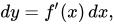
In calculus, the differential represents the principal part of the change in a function with respect to changes in the independent variable. The differential is defined by where is the derivative of f with respect to , and is an additional real variable (so that is a function of and ). The notation is such that the equation

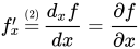
holds, where the derivative is represented in the Leibniz notation , and this is consistent with regarding the derivative as the quotient of the differentials. One also writes


The precise meaning of the variables and depends on the context of the application and the required level of mathematical rigor. The domain of these variables may take on a particular geometrical significance if the differential is regarded as a particular differential form, or analytical significance if the differential is regarded as a linear approximation to the increment of a function. Traditionally, the variables and are considered to be very small (infinitesimal), and this interpretation is made rigorous in non-standard analysis.

History and usage

[edit]

The differential was first introduced via an intuitive or heuristic definition by Isaac Newton and furthered by Gottfried Leibniz, who thought of the differential dy as an infinitely small (or infinitesimal) change in the value y of the function, corresponding to an infinitely small change dx in the function's argument x. For that reason, the instantaneous rate of change of y with respect to x, which is the value of the derivative of the function, is denoted by the fraction

in what is called the Leibniz notation for derivatives. The quotient is not infinitely small; rather it is a real number.

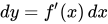
The use of infinitesimals in this form was widely criticized, for instance by the famous pamphlet The Analyst by Bishop Berkeley. Augustin-Louis Cauchy (1823) defined the differential without appeal to the atomism of Leibniz's infinitesimals.[1][2] Instead, Cauchy, following d'Alembert, inverted the logical order of Leibniz and his successors: the derivative itself became the fundamental object, defined as a limit of difference quotients, and the differentials were then defined in terms of it. That is, one was free to define the differential by an expression in which and are simply new variables taking finite real values,[3] not fixed infinitesimals as they had been for Leibniz.[4]
According to Boyer (1959, p. 12), Cauchy's approach was a significant logical improvement over the infinitesimal approach of Leibniz because, instead of invoking the metaphysical notion of infinitesimals, the quantities and could now be manipulated in exactly the same manner as any other real quantities in a meaningful way. Cauchy's overall conceptual approach to differentials remains the standard one in modern analytical treatments,[5] although the final word on rigor, a fully modern notion of the limit, was ultimately due to Karl Weierstrass.[6]

In physical treatments, such as those applied to the theory of thermodynamics, the infinitesimal view still prevails. Courant & John (1999, p. 184) reconcile the physical use of infinitesimal differentials with the mathematical impossibility of them as follows. The differentials represent finite non-zero values that are smaller than the degree of accuracy required for the particular purpose for which they are intended. Thus "physical infinitesimals" need not appeal to a corresponding mathematical infinitesimal in order to have a precise sense.

Following twentieth-century developments in mathematical analysis and differential geometry, it became clear that the notion of the differential of a function could be extended in a variety of ways. In real analysis, it is more desirable to deal directly with the differential as the principal part of the increment of a function. This leads directly to the notion that the differential of a function at a point is a linear functional of an increment . This approach allows the differential (as a linear map) to be developed for a variety of more sophisticated spaces, ultimately giving rise to such notions as the Fréchet or Gateaux derivative. Likewise, in differential geometry, the differential of a function at a point is a linear function of a tangent vector (an "infinitely small displacement"), which exhibits it as a kind of one-form: the exterior derivative of the function. In non-standard calculus, differentials are regarded as infinitesimals, which can themselves be put on a rigorous footing (see differential (infinitesimal)).

Definition

[edit]
The differential of a function at a point .

The differential is defined in modern treatments of differential calculus as follows.[7] The differential of a function of a single real variable is the function of two independent real variables and given by


One or both of the arguments may be suppressed, i.e., one may see or simply . If , the differential may also be written as . Since , it is conventional to write so that the following equality holds:


This notion of differential is broadly applicable when a linear approximation to a function is sought, in which the value of the increment is small enough. More precisely, if is a differentiable function at , then the difference in -values

satisfies

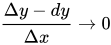
where the error in the approximation satisfies as . In other words, one has the approximate identity

in which the error can be made as small as desired relative to by constraining to be sufficiently small; that is to say, as . For this reason, the differential of a function is known as the principal (linear) part in the increment of a function: the differential is a linear function of the increment , and although the error may be nonlinear, it tends to zero rapidly as tends to zero.
Differentials in several variables

[edit]
Operator / Function
Differential 1: 2:

3:

Partial derivative
Total derivative

Following Goursat (1904, I, §15), for functions of more than one independent variable,

the partial differential of y with respect to any one of the variables xi is the principal part of the change in y resulting from a change dxi in that one variable. The partial differential is therefore

involving the partial derivative of y with respect to xi. The sum of the partial differentials with respect to all of the independent variables is the total differential

which is the principal part of the change in y resulting from changes in the independent variables xi.

More precisely, in the context of multivariable calculus, following Courant (1937b), if f is a differentiable function, then by the definition of differentiability, the increment

where the error terms ε i tend to zero as the increments Δxi jointly tend to zero. The total differential is then rigorously defined as

Since, with this definition, one has


As in the case of one variable, the approximate identity holds

in which the total error can be made as small as desired relative to by confining attention to sufficiently small increments.

Application of the total differential to error estimation

[edit]

In measurement, the total differential is used in estimating the error of a function based on the errors of the parameters . Assuming that the interval is short enough for the change to be approximately linear:

and that all variables are independent, then for all variables,

This is because the derivative with respect to the particular parameter gives the sensitivity of the function to a change in , in particular the error . As they are assumed to be independent, the analysis describes the worst-case scenario. The absolute values of the component errors are used, because after simple computation, the derivative may have a negative sign. From this principle the error rules of summation, multiplication etc. are derived, e.g.:

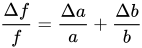
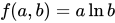
Let . Then, the finite error can be approximated as

Evaluating the derivatives: Dividing by f, which is a × b

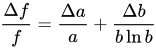
That is to say, in multiplication, the total relative error is the sum of the relative errors of the parameters.

To illustrate how this depends on the function considered, consider the case where the function is instead. Then, it can be computed that the error estimate is with an extra ln b factor not found in the case of a simple product. This additional factor tends to make the error smaller, as the denominator b ln b is larger than a bare b.
Higher-order differentials

[edit]

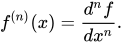
Higher-order differentials of a function y = f(x) of a single variable x can be defined via:[8] and, in general, Informally, this motivates Leibniz's notation for higher-order derivatives When the independent variable x itself is permitted to depend on other variables, then the expression becomes more complicated, as it must include also higher order differentials in x itself. Thus, for instance, and so forth.


Similar considerations apply to defining higher order differentials of functions of several variables. For example, if f is a function of two variables x and y, then where is a binomial coefficient. In more variables, an analogous expression holds, but with an appropriate multinomial expansion rather than binomial expansion.[9]

Higher order differentials in several variables also become more complicated when the independent variables are themselves allowed to depend on other variables. For instance, for a function f of x and y which are allowed to depend on auxiliary variables, one has

Because of this notational awkwardness, the use of higher order differentials was roundly criticized by Hadamard (1935), who concluded:

Enfin, que signifie ou que représente l'égalité

A mon avis, rien du tout.

That is: Finally, what is meant, or represented, by the equality [...]? In my opinion, nothing at all. In spite of this skepticism, higher order differentials did emerge as an important tool in analysis.[10]

In these contexts, the n-th order differential of the function f applied to an increment Δx is defined by or an equivalent expression, such as where is an nth forward difference with increment tΔx.

This definition makes sense as well if f is a function of several variables (for simplicity taken here as a vector argument). Then the n-th differential defined in this way is a homogeneous function of degree n in the vector increment Δx. Furthermore, the Taylor series of f at the point x is given by The higher order Gateaux derivative generalizes these considerations to infinite dimensional spaces.

Properties

[edit]

A number of properties of the differential follow in a straightforward manner from the corresponding properties of the derivative, partial derivative, and total derivative. These include:[11]

  • Linearity: For constants a and b and differentiable functions f and g,
  • Product rule: For two differentiable functions f and g,

An operation d with these two properties is known in abstract algebra as a derivation. They imply the power rule In addition, various forms of the chain rule hold, in increasing level of generality:[12]

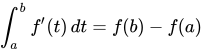
  • If y = f(u) is a differentiable function of the variable u and u = g(x) is a differentiable function of x, then
  • If y = f(x1, ..., xn) and all of the variables x1, ..., xn depend on another variable t, then by the chain rule for partial derivatives, one has Heuristically, the chain rule for several variables can itself be understood by dividing through both sides of this equation by the infinitely small quantity dt.
  • More general analogous expressions hold, in which the intermediate variables xi depend on more than one variable.

General formulation

[edit]

A consistent notion of differential can be developed for a function f : RnRm between two Euclidean spaces. Let xxRn be a pair of Euclidean vectors. The increment in the function f is If there exists an m × n matrix A such that in which the vector ε → 0 as Δx → 0, then f is by definition differentiable at the point x. The matrix A is sometimes known as the Jacobian matrix, and the linear transformation that associates to the increment ΔxRn the vector AΔxRm is, in this general setting, known as the differential df(x) of f at the point x. This is precisely the Fréchet derivative, and the same construction can be made to work for a function between any Banach spaces.

Another fruitful point of view is to define the differential directly as a kind of directional derivative: which is the approach already taken for defining higher order differentials (and is most nearly the definition set forth by Cauchy). If t represents time and x position, then h represents a velocity instead of a displacement as we have heretofore regarded it. This yields yet another refinement of the notion of differential: that it should be a linear function of a kinematic velocity. The set of all velocities through a given point of space is known as the tangent space, and so df gives a linear function on the tangent space: a differential form. With this interpretation, the differential of f is known as the exterior derivative, and has broad application in differential geometry because the notion of velocities and the tangent space makes sense on any differentiable manifold. If, in addition, the output value of f also represents a position (in a Euclidean space), then a dimensional analysis confirms that the output value of df must be a velocity. If one treats the differential in this manner, then it is known as the pushforward since it "pushes" velocities from a source space into velocities in a target space.

Other approaches

[edit]

Although the notion of having an infinitesimal increment dx is not well-defined in modern mathematical analysis, a variety of techniques exist for defining the infinitesimal differential so that the differential of a function can be handled in a manner that does not clash with the Leibniz notation. These include:

Examples and applications

[edit]

Differentials may be effectively used in numerical analysis to study the propagation of experimental errors in a calculation, and thus the overall numerical stability of a problem (Courant 1937a). Suppose that the variable x represents the outcome of an experiment and y is the result of a numerical computation applied to x. The question is to what extent errors in the measurement of x influence the outcome of the computation of y. If the x is known to within Δx of its true value, then Taylor's theorem gives the following estimate on the error Δy in the computation of y: where ξ = x + θΔx for some 0 < θ < 1. If Δx is small, then the second order term is negligible, so that Δy is, for practical purposes, well-approximated by dy = f'(x) Δx.

The differential is often useful to rewrite a differential equation in the form in particular when one wants to separate the variables.

Notes

[edit]

See also

[edit]

References

[edit]
[edit]
Revisions and contributorsEdit on WikipediaRead on Wikipedia
from Grokipedia
In calculus, the differential of a function provides a linear approximation to the change in the function's value resulting from small changes in its input variables, expressed as $ df = f'(x) , dx $ for a single-variable function $ f(x) $, where $ f'(x) $ is the derivative and $ dx $ represents an infinitesimal or small increment in $ x $.[1] This concept, distinct from the derivative itself, quantifies the principal part of the function's variation and serves as the foundation for more advanced topics in analysis and geometry.[2] For functions of a single variable, the differential $ dy $ approximates the actual change $ \Delta y $ in $ y = f(x) $ when $ x $ changes by a small amount $ \Delta x $, such that $ dy = f'(x) , dx $ with $ dx = \Delta x $, and the approximation improves as $ dx $ approaches zero.[1] This formulation arises naturally from the definition of the derivative as a limit and is used in applications like error estimation, where the maximum error in a quantity, such as the volume of a sphere with radius $ r $ and small error $ \Delta r $, can be bounded using $ dV = 4\pi r^2 , dr $.[1] In multivariable calculus, the differential extends to functions $ f(x_1, x_2, \dots, x_n) $ as $ df = \sum_{i=1}^n \frac{\partial f}{\partial x_i} , dx_i $, or equivalently in vector form $ df = \nabla f \cdot d\mathbf{r} $, where $ \nabla f $ is the gradient vector and $ d\mathbf{r} $ is the vector of input differentials.[3] This linear map captures the function's behavior near a point via the tangent plane (in two variables) or hyperplane (in higher dimensions), requiring the partial derivatives to exist and the function to be differentiable, which implies continuity.[3] For example, for $ f(x, y) = x^2 y^3 $, the differential is $ df = 2xy^3 , dx + 3x^2 y^2 , dy $.[2] The differential's utility spans optimization, where it aids in identifying critical points through the condition $ df = 0 $; error propagation in measurements, bounding changes via $ |\Delta f| \leq \sum |\frac{\partial f}{\partial x_i}| |\Delta x_i| $; and coordinate transformations, such as converting between Cartesian and polar systems using $ dx = \cos \theta , dr - r \sin \theta , d\theta $ and $ dy = \sin \theta , dr + r \cos \theta , d\theta $.[3][2] In differential geometry, it represents the pushforward of tangent vectors, linking local linear approximations to global manifold structures.[2] Higher-order differentials, like $ d^2 f = \sum \frac{\partial^2 f}{\partial x_i \partial x_j} , dx_i , dx_j $, further enable Taylor series expansions for more precise approximations.[3]

Historical Development and Usage

Origins and Evolution

The concept of the differential originated in the late 17th century as part of the emerging calculus, primarily through the work of Gottfried Wilhelm Leibniz. In his 1684 publication "Nova Methodus pro Maximis et Minimis, itemque Tangentibus" in Acta Eruditorum, Leibniz introduced differentials as infinitesimal changes, denoted by symbols such as dxdx and dydy, representing arbitrarily small increments in the independent and dependent variables, respectively.[4] These notations allowed for the systematic calculation of tangents, maxima, and minima by treating differentials as actual though evanescent quantities, with rules like d(x+y)=dx+dyd(x + y) = dx + dy and d(xy)=xdy+ydxd(xy) = x\, dy + y\, dx.[5] Leibniz's approach framed differentials as a heuristic tool for infinitesimal analysis, marking the birth of differential calculus as a distinct method.[6] Independently, Isaac Newton developed a parallel framework in the 1660s, known as the method of fluxions, where rates of change were conceptualized through "moments" or infinitesimal quantities akin to differentials, though he employed dot notation for derivatives rather than Leibniz's symbols.[7] Newton's De Methodis Serierum et Fluxionum (written 1671, published 1736) refined these ideas by linking fluxions to the inverse process of integration, amid growing debates over the philosophical validity of infinitesimals, which critics like George Berkeley later derided as logically inconsistent "ghosts of departed quantities."[7] Leonhard Euler further advanced the concept in the 18th century through his Institutiones Calculi Differentialis (1755), integrating Leibnizian differentials with Newtonian fluxions into a more systematic treatment of analysis; he explored differentiation under variable substitutions, finite differences, and applications to differential equations, while defending the utility of infinitesimals against skepticism by emphasizing their operational effectiveness in computations.[8] Augustin-Louis Cauchy contributed to refining differentials in the early 19th century with his Cours d'Analyse de l'École Royale Polytechnique (1821), where he introduced a more precise notion of limits to underpin convergence and continuity, laying groundwork for interpreting differentials without direct reliance on undefined infinitesimals.[9] This work addressed ongoing controversies by providing analytic rigor to calculus foundations. The full rigorization came later in the century through Karl Weierstrass, whose lectures around 1858–1861 on the introduction to analysis replaced infinitesimals entirely with limit-based definitions, conceptualizing the differential as the linear approximation given by the derivative times the increment, thus transforming it from a heuristic infinitesimal into a precise mathematical object in real analysis.[10] This evolution elevated differentials from a contentious tool in early calculus to a cornerstone of modern mathematical analysis.[11]

Modern Interpretations and Applications

In contemporary mathematics and applied sciences, the differential of a function plays a pivotal role in optimization by providing the gradient, which indicates the direction of steepest ascent or descent for an objective function. Gradient-based methods, such as gradient descent, rely on these differentials to iteratively refine solutions in numerical optimization problems, enabling efficient convergence in convex settings. This framework is essential for solving large-scale problems where analytical solutions are infeasible. In machine learning, differentials underpin gradient computation in algorithms like backpropagation, which propagates infinitesimal changes in the loss function backward through neural network layers to update parameters via the chain rule. This process, formalized in seminal work on multilayer perceptrons, allows for scalable training of deep networks by computing exact partial derivatives efficiently.[12] Automatic differentiation further extends this by algorithmically evaluating differentials of complex programs, supporting reverse-mode accumulation for high-dimensional parameter spaces in modern AI models.[13] Physics employs differentials to model infinitesimal state changes, notably in thermodynamics where the work differential is expressed as
dW=PdV dW = P \, dV
for reversible pressure-volume processes, capturing energy transfers in quasi-static systems.[14] In engineering, differentials facilitate sensitivity analysis by quantifying how small parameter perturbations propagate through differential equations, informing robust design in structural and mechanical systems.[15] Similarly, in control theory, linearized differentials around operating points enable stability assessments and optimal control synthesis for dynamic systems governed by ordinary differential equations.[16]

Fundamental Definition in One Variable

Precise Mathematical Definition

In single-variable calculus, the concept of the differential presupposes that the function f:RRf: \mathbb{R} \to \mathbb{R} is differentiable at a point aa, meaning the derivative f(a)f'(a) exists as the limit limh0f(a+h)f(a)h\lim_{h \to 0} \frac{f(a + h) - f(a)}{h}.[17] This differentiability condition ensures that the function's behavior near aa can be captured by a linear approximation derived from first principles.[18] The precise mathematical definition of the differential dfdf at aa is df=f(a)dxdf = f'(a) \, dx, where dxdx is an arbitrary real increment in the independent variable.[17] This expression represents the principal part of the change in ff, treating f(a)f'(a) as the scaling factor for the increment dxdx. For a function y=f(x)y = f(x), the notation is commonly dy=f(x)dxdy = f'(x) \, dx.[19][20] This definition arises from the limit characterization of differentiability. Specifically, ff is differentiable at aa if there exists a linear function L(h)=f(a)hL(h) = f'(a) h such that limh0f(a+h)f(a)L(h)h=0\lim_{h \to 0} \frac{f(a + h) - f(a) - L(h)}{h} = 0.[18] Equivalently, f(a+h)=f(a)+f(a)h+r(h)f(a + h) = f(a) + f'(a) h + r(h), where r(h)/h0r(h)/h \to 0 as h0h \to 0 (i.e., r(h)=o(h)r(h) = o(h)). Setting h=dxh = dx and identifying df=f(a)dxdf = f'(a) \, dx yields the differential as the linear term in this expansion.[17][18] For small increments Δx\Delta x, the differential provides the best linear approximation to the actual change Δf=f(a+Δx)f(a)\Delta f = f(a + \Delta x) - f(a), so Δfdf\Delta f \approx df with the error term satisfying Δfdf=o(Δx)\Delta f - df = o(\Delta x) as Δx0\Delta x \to 0.[19] This approximation underpins the utility of differentials in estimating function changes near aa.[20]

Intuitive and Geometric Meaning

The differential of a function provides an intuitive way to understand local changes in the function's value through the lens of its graph as a curve in the plane. For a function y=f(x)y = f(x), the differential dfdf represents the infinitesimal change in yy corresponding to an infinitesimal change dxdx in xx, which geometrically corresponds to the vertical rise along the tangent line to the curve at a point, rather than the actual arc length along the curve itself.[21] This tangent line serves as the best linear approximation to the curve near that point, capturing the function's behavior over a small neighborhood where the curve appears nearly straight.[22] Geometrically, consider points P(x,f(x))P(x, f(x)) and Q(x+Δx,f(x+Δx))Q(x + \Delta x, f(x + \Delta x)) on the graph; the secant line connecting them has a slope that approaches the tangent slope f(x)f'(x) as Δx\Delta x approaches zero, and the corresponding vertical change Δy\Delta y along the secant converges to df=f(x)dxdf = f'(x) \, dx along the tangent.[21] Here, dxdx scales the input perturbation, while dfdf scales the output response, emphasizing the differential's role in linearizing the nonlinear function locally for estimation purposes. This approximation is particularly useful in contexts where computing the full change Δy\Delta y is impractical, as it allows quick estimates using only the tangent slope without reevaluating the function at nearby points.[22] For non-mathematical audiences, the concept aligns with everyday notions of instantaneous rates, such as speed: if s(t)s(t) is the distance traveled at time tt, then the differential ds=vdtds = v \, dt approximates the small distance covered in a tiny time interval dtdt using the instantaneous velocity vv, mirroring how the tangent to the distance-time graph gives the speed at that instant.[22] This perspective highlights why differentials are valuable for modeling real-world approximations, like error propagation or optimization, by focusing on scaled linear changes rather than exact computations.[21]

Extension to Multiple Variables

Total Differential Formulation

The total differential formulation extends the differential concept from functions of a single variable to those of multiple variables, assuming the function is differentiable at the point of interest, which requires the partial derivatives to exist in a neighborhood and satisfy the differentiability condition. In the single-variable case, the differential df approximates the change in f as f'(x) dx; similarly, for multivariable functions, it captures the combined effect of independent increments in each input variable through partial derivatives.[23] For a function $ f: \mathbb{R}^2 \to \mathbb{R} $ of two variables, such as $ f(x, y) $, the total differential at a point $ (x, y) $ is defined as
df=fxdx+fydy, df = \frac{\partial f}{\partial x} \, dx + \frac{\partial f}{\partial y} \, dy,
where $ dx $ and $ dy $ are independent infinitesimal increments in the input variables. This expression arises from the requirement that the partial derivatives $ \frac{\partial f}{\partial x} $ and $ \frac{\partial f}{\partial y} $ exist, providing the rates of change with respect to each variable while holding the other constant.[23][24] In the general case of a function $ f: \mathbb{R}^n \to \mathbb{R} $, the total differential is the sum of contributions from each variable:
df=i=1nfxidxi, df = \sum_{i=1}^n \frac{\partial f}{\partial x_i} \, dx_i,
with $ dx_i $ denoting the independent increments in the $ i $-th variable $ x_i $, and all partial derivatives $ \frac{\partial f}{\partial x_i} $ assumed to exist. This formulation treats the inputs as varying independently, allowing the total change in $ f $ to be decomposed into partial changes along each coordinate direction.[23][25] The total differential df serves as a linear map that approximates the change in the output $ f $ induced by a vector of input changes $ d\mathbf{x} = (dx_1, \dots, dx_n)^T $. In matrix notation, this is expressed using the gradient vector $ \nabla f = \left( \frac{\partial f}{\partial x_1}, \dots, \frac{\partial f}{\partial x_n} \right) $, yielding
df=fdx, df = \nabla f \cdot d\mathbf{x},
where $ \nabla f $ forms the rows of the Jacobian matrix for the scalar-valued function (a $ 1 \times n $ matrix). This linear approximation captures the first-order behavior of $ f $ near the point, with the Jacobian providing the transformation from input increments to the output differential.[26][27]

Error Analysis Using Differentials

In error analysis, the total differential of a multivariable function f(x)f(\mathbf{x}), where x=(x1,,xn)\mathbf{x} = (x_1, \dots, x_n), provides a linear approximation for estimating the change Δf\Delta f in the function value due to small changes Δxi\Delta x_i in the inputs. For small errors, the absolute error is approximated as Δfdf=i=1nfxiΔxi|\Delta f| \approx |df| = \left| \sum_{i=1}^n \frac{\partial f}{\partial x_i} \Delta x_i \right|, where the partial derivatives are evaluated at the nominal values of x\mathbf{x}.[28] This approximation arises from the first-order Taylor expansion, treating the differential dfdf as the best linear estimate of the function's variation.[29] To obtain a conservative upper bound on the error, the triangle inequality is applied, yielding the maximum possible error dfi=1nfxiΔxi|df| \leq \sum_{i=1}^n \left| \frac{\partial f}{\partial x_i} \right| |\Delta x_i|. This bound assumes the worst-case scenario where all error contributions add constructively, which is useful in engineering and experimental contexts to ensure safety margins.[28] It provides a straightforward way to propagate maximum allowable errors without assuming probabilistic distributions for the Δxi\Delta x_i. A practical application appears in physical measurements, such as estimating the uncertainty in the volume of a sphere V=43πr3V = \frac{4}{3} \pi r^3 given an error in the radius rr. Here, the partial derivative Vr=4πr2\frac{\partial V}{\partial r} = 4 \pi r^2, so the propagated error is ΔV4πr2Δr\Delta V \approx 4 \pi r^2 \Delta r. For instance, if r=3.00×10³r = 3.00 \times 10^{-3} m with Δr=0.03×10³\Delta r = 0.03 \times 10^{-3} m, then V1.131×107V \approx 1.131 \times 10^{-7} m³ and ΔV3.4×109\Delta V \approx 3.4 \times 10^{-9} m³, corresponding to a relative error amplification from 1% in radius to 3% in volume.[1] In statistical contexts, where errors are random and independent with standard deviations σxi\sigma_{x_i}, the differentials enable propagation of uncertainty via the root-sum-square formula for the variance: σf2i=1n(fxiσxi)2\sigma_f^2 \approx \sum_{i=1}^n \left( \frac{\partial f}{\partial x_i} \sigma_{x_i} \right)^2, so the standard deviation is σfi=1n(fxiσxi)2\sigma_f \approx \sqrt{ \sum_{i=1}^n \left( \frac{\partial f}{\partial x_i} \sigma_{x_i} \right)^2 }. This method, often called the delta method, quantifies the propagated standard deviation assuming Gaussian-like errors and linearity.[29] The validity of these differential-based approximations relies on the errors Δxi\Delta x_i being sufficiently small relative to the scale over which ff is approximately linear, typically ensuring second-order terms in the Taylor expansion remain negligible. For non-small errors, the linear estimate under- or over-predicts the true change, potentially leading to inaccurate bounds; in such cases, higher-order methods or numerical simulations are required, though differentials remain a foundational tool for initial assessments.[28]

Advanced Extensions

Higher-Order Differentials

Higher-order differentials extend the concept of the first differential to capture nonlinear aspects of function behavior through successive applications of the differential operator. For a differentiable function ff, the second differential is defined as d2f=d(df)d^2 f = d(df), where dfdf is the first differential, and higher-order differentials dkfd^k f for k2k \geq 2 are obtained recursively by applying the differential to the previous order.[3] This recursive structure allows for the analysis of curvature and higher-degree approximations in both single and multivariable settings.[30] In the case of a function f:RRf: \mathbb{R} \to \mathbb{R} that is twice continuously differentiable, the second differential simplifies to d2f(x)=f(x)(dx)2d^2 f(x) = f''(x) (dx)^2, representing the infinitesimal quadratic change in ff.[31] For higher orders, dkf(x)=f(k)(x)(dx)kd^k f(x) = f^{(k)}(x) (dx)^k, where f(k)f^{(k)} denotes the kk-th derivative, assuming sufficient smoothness.[3] This form highlights the homogeneity of degree kk in the increments dxdx, distinguishing it from the linear nature of the first-order differential df=f(x)dxdf = f'(x) dx. For functions f:RnRf: \mathbb{R}^n \to \mathbb{R} with continuous second partial derivatives, the second differential is a quadratic form given by
d2f(x)=i=1nj=1n2fxixj(x)dxidxj, d^2 f(\mathbf{x}) = \sum_{i=1}^n \sum_{j=1}^n \frac{\partial^2 f}{\partial x_i \partial x_j}(\mathbf{x}) \, dx_i \, dx_j,
which corresponds to the bilinear form associated with the Hessian matrix Hij=2fxixjH_{ij} = \frac{\partial^2 f}{\partial x_i \partial x_j}.[30] Higher-order differentials follow similarly, with the kk-th differential involving the kk-th partial derivatives and products of the dxidx_i.[3]
The recursive computation of higher-order differentials relies on applying the total differential operator d=idxixid = \sum_i dx_i \frac{\partial}{\partial x_i} to the expression from the previous order, treating differentials like dxidx_i as constants.[31] For mixed partials in the second differential, Clairaut's theorem ensures that 2fxixj=2fxjxi\frac{\partial^2 f}{\partial x_i \partial x_j} = \frac{\partial^2 f}{\partial x_j \partial x_i} provided the second partials are continuous, allowing symmetric treatment in the summation without regard to differentiation order.[3] This equality simplifies explicit calculations, as the coefficient of dxidxjdx_i dx_j for iji \neq j is twice the mixed partial in the quadratic form. Unlike finite differences, which approximate changes over finite increments and accumulate truncation errors, higher-order differentials are exact infinitesimal approximations that are linear (or homogeneous) in the differentials at each order, providing precise local information without discretization. This infinitesimal perspective maintains validity for arbitrarily small changes, emphasizing conceptual linearity in the tangent space rather than numerical computation.[30]

Relation to Taylor Expansions

Taylor's theorem provides a fundamental connection between higher-order differentials and the local approximation of functions through polynomial expansions. For a function f:RRf: \mathbb{R} \to \mathbb{R} that is n+1n+1 times differentiable at a point aa, the theorem states that
f(a+h)=f(a)+df+12!d2f++1n!dnf+Rn(h), f(a + h) = f(a) + df + \frac{1}{2!} d^2 f + \cdots + \frac{1}{n!} d^n f + R_n(h),
where df=f(a)dhdf = f'(a) \, dh, dkf=f(k)(a)dhkd^k f = f^{(k)}(a) \, dh^k for k2k \geq 2, and Rn(h)R_n(h) is the remainder term.[32] This formulation interprets each term 1k!dkf\frac{1}{k!} d^k f as the kk-th order contribution to the approximation, capturing the function's behavior up to infinitesimal changes of order hkh^k.[33] In the multivariable setting, for a function f:URmRf: U \subseteq \mathbb{R}^m \to \mathbb{R} that is CpC^p on an open set UU, Taylor's theorem extends using higher derivatives as symmetric multilinear maps. The expansion becomes
f(a+h)=j=0pDjf(a)j!(h,,h)+Rp,a(h), f(a + h) = \sum_{j=0}^p \frac{D^j f(a)}{j!} (h, \dots, h) + R_{p,a}(h),
where Djf(a)D^j f(a) is the jj-th derivative, a multilinear form on (Rm)j(\mathbb{R}^m)^j, and the term Djf(a)j!(h(j))\frac{D^j f(a)}{j!} (h^{(j)}) arises from the higher-order differential djfd^j f.[32][34] This structure allows the approximation to incorporate interactions among variables through partial derivatives in the multilinear forms. The remainder Rn(h)R_n(h) plays a crucial role in assessing convergence of the series and estimating approximation errors. In the Lagrange form, for the one-variable case, Rn(h)=f(n+1)(c)(n+1)!hn+1R_n(h) = \frac{f^{(n+1)}(c)}{(n+1)!} h^{n+1} for some cc between aa and a+ha+h, providing a bound on the truncation error based on the (n+1)(n+1)-th derivative.[35] Similar integral or Lagrange forms apply in multiple variables, ensuring the remainder is O(hn+1)O(\|h\|^{n+1}) as h0h \to 0.[32] In numerical analysis, these expansions quantify truncation errors in methods like finite differences, where approximating derivatives via Taylor series leads to error terms of higher order in the step size, guiding the choice of discretization for accuracy.[36]

Algebraic Properties

Linearity and Basic Operations

The differential of a function exhibits linearity as an algebraic operation on linear combinations of functions. For differentiable functions ff and gg, and scalar constants aa and bb, the differential satisfies d(af+bg)=adf+bdgd(af + bg) = a\, df + b\, dg.[37] This property arises directly from the definition of the differential as a linear map, where the derivative Df(a)Df(a) is a linear transformation, ensuring additivity D(f+g)(a)=Df(a)+Dg(a)D(f + g)(a) = Df(a) + Dg(a) and homogeneity D(cf)(a)=cDf(a)D(cf)(a) = c\, Df(a).[38] In addition, the differential dfdf is linear with respect to the input increments dxdx. For a function f:RnRf: \mathbb{R}^n \to \mathbb{R}, df=i=1nfxidxidf = \sum_{i=1}^n \frac{\partial f}{\partial x_i} dx_i, which is additive in the dxidx_i (i.e., d(f1+f2)=df1+df2d(f_1 + f_2) = df_1 + df_2) and homogeneous (i.e., d(cf)=cdfd(cf) = c\, df for scalar cc).[37] This linearity in dxdx reflects the first-order approximation of ff near a point, where changes in the function scale proportionally with changes in the variables.[38] Basic operations on products and related forms follow from the product rule for differentials. For differentiable functions ff and gg, d(fg)=fdg+gdfd(fg) = f\, dg + g\, df.[37] This can be extended to derive the quotient rule, d(fg)=gdffdgg2d\left(\frac{f}{g}\right) = \frac{g\, df - f\, dg}{g^2} (assuming g0g \neq 0), and the power rule for integer powers, such as d(fn)=nfn1dfd(f^n) = n f^{n-1} df, through repeated application of the product rule.[38] These rules maintain the linear structure while handling multiplicative compositions. For higher-order differentials, bilinearity emerges in the second differential d2fd^2 f, which is a symmetric bilinear form in the increments. Specifically, d2f=i=1nj=1n2fxixjdxidxjd^2 f = \sum_{i=1}^n \sum_{j=1}^n \frac{\partial^2 f}{\partial x_i \partial x_j} dx_i dx_j, linear in each dxkdx_k separately.[39] For a product fgfg, the second differential includes cross terms: d2(fg)=fd2g+gd2f+2dfdgd^2(fg) = f\, d^2 g + g\, d^2 f + 2\, df\, dg, capturing interactions between the first differentials of ff and gg.[38] This bilinearity follows the Leibniz rule for higher derivatives, generalizing the first-order product rule. These properties can be proven from the definition of the differential as the best linear approximation and the chain rule for compositions. For instance, linearity in functions follows by applying the limit definition to sums and scalar multiples, while the product rule derives from considering fgfg as a composition with multiplication.[37] Invariance under variable substitution holds because the differential transforms covariantly via the chain rule: if x=x(u)x = x(u), then df=fukdukdf = \sum \frac{\partial f}{\partial u_k} du_k, preserving the linear approximation regardless of the coordinate system.[38]

Differentiation Rules for Differentials

The chain rule for differentials in the single-variable case arises directly from the standard chain rule for derivatives. If $ y = f(u) $ where $ u $ is a function of an independent variable, the differential of $ y $ is given by
dy=dydudu, dy = \frac{dy}{du} \, du,
where $ \frac{dy}{du} $ is the derivative of $ f $ evaluated at $ u $. This formulation follows from the definition of the differential as $ dy = f'(u) , du $, mirroring the derivative chain rule $ \frac{dy}{dx} = \frac{dy}{du} \cdot \frac{du}{dx} $ by substituting $ du = \frac{du}{dx} , dx $.[40] This rule extends naturally to multivariable functions. For a scalar-valued function $ f: \mathbb{R}^n \to \mathbb{R} $, the total differential is
df=fdu, df = \nabla f \cdot d\mathbf{u},
where $ \nabla f $ is the gradient vector of $ f $ and $ d\mathbf{u} $ is the differential vector of the input variables. In the case of two variables, if $ z = f(x, y) $, then
dz=zxdx+zydy. dz = \frac{\partial z}{\partial x} \, dx + \frac{\partial z}{\partial y} \, dy.
This multivariable form derives from the chain rule applied to compositions where the intermediate variables depend on a parameter, such as $ x = x(t) $ and $ y = y(t) $, yielding $ dz = \frac{\partial z}{\partial x} \frac{dx}{dt} dt + \frac{\partial z}{\partial y} \frac{dy}{dt} dt $, which simplifies to the dot product expression upon identifying the differentials.[41] For inverse functions, the differential rule follows from the reciprocal nature of derivatives. If $ x = g(y) $ is the inverse of $ y = f(x) $, then
dx=dxdydy, dx = \frac{dx}{dy} \, dy,
where $ \frac{dx}{dy} = \frac{1}{\frac{dy}{dx}} = \frac{1}{f'(x)} $, evaluated at the corresponding point. This is obtained by differentiating $ x = g(y) $ with respect to $ y $ and using the chain rule on the inverse relation $ y = f(g(y)) $, which implies $ 1 = f'(g(y)) \cdot \frac{dg}{dy} $.[42] Implicit differentiation using differentials applies to relations defined by $ F(x, y) = 0 $, where $ y $ is implicitly a function of $ x $. Differentiating both sides gives $ dF = 0 $, so
Fxdx+Fydy=0, \frac{\partial F}{\partial x} \, dx + \frac{\partial F}{\partial y} \, dy = 0,
which rearranges to $ dy = -\frac{\frac{\partial F}{\partial x}}{\frac{\partial F}{\partial y}} , dx $. This rule stems from the total differential of $ F $ and the assumption that $ dF = 0 $ along the implicit curve, extending the single-variable chain rule to treat $ y $ as dependent on $ x $.[43] Logarithmic differentiation simplifies computations for products, quotients, and powers by leveraging the differential of the natural logarithm. For a positive function $ f $,
d(lnf)=1fdf, d(\ln f) = \frac{1}{f} \, df,
or equivalently, $ df = f , d(\ln f) $. To apply this, take $ \ln y = \ln f(x) $, differentiate both sides to obtain $ \frac{1}{y} dy = d(\ln f) $, and multiply through by $ y $ to isolate $ dy $. This technique derives from the chain rule applied to the composition $ \ln \circ f $, reducing complex expressions via logarithmic properties like $ \ln(ab) = \ln a + \ln b $.[44]

Abstract and General Frameworks

Formulation in Vector Spaces

In the context of functions between normed vector spaces, the differential of a function f:VWf: V \to W, where VV and WW are normed spaces over the real or complex numbers, is generalized through the notion of the Fréchet derivative. At a point aVa \in V, the differential dfa:VWdf_a: V \to W is defined as dfa(h)=Df(a)(h)df_a(h) = Df(a)(h), where Df(a)Df(a) is a bounded linear operator that provides the best linear approximation to the increment f(a+h)f(a)f(a + h) - f(a) for small hVh \in V. This approximation captures the local linear behavior of ff near aa, extending the classical differential from single-variable calculus to infinite-dimensional settings.[45] The Fréchet derivative Df(a)Df(a) exists if there is a bounded linear operator L:VWL: V \to W such that
limh0f(a+h)f(a)L(h)WhV=0. \lim_{\|h\| \to 0} \frac{\|f(a + h) - f(a) - L(h)\|_W}{\|h\|_V} = 0.
Here, the limit condition ensures that the error in the linear approximation is negligible compared to h\|h\|, making LL the unique such operator when it exists. This definition applies to general normed spaces but is particularly powerful in Banach spaces, where completeness allows for deeper analytic results, such as the implicit function theorem in infinite dimensions.[45] A related but weaker concept is the Gâteaux derivative, which considers directional approximations. The Gâteaux derivative at aa in the direction hVh \in V is given by
DGf(a)(h)=limt0f(a+th)f(a)t, D_G f(a)(h) = \lim_{t \to 0} \frac{f(a + t h) - f(a)}{t},
provided the limit exists for all hh. If the Fréchet derivative exists, then the Gâteaux derivative exists and coincides with it, but the converse does not hold in general, as the Gâteaux derivative may fail to be uniformly approximated across all directions. This distinction is crucial in Banach spaces, where Fréchet differentiability implies stronger uniformity than Gâteaux differentiability.[45] For linear maps, the Fréchet derivative simplifies significantly. If f:VWf: V \to W is a bounded linear operator, then Df(a)=fDf(a) = f for all aVa \in V, since f(a+h)f(a)=f(h)f(a + h) - f(a) = f(h) exactly satisfies the limit condition with L=fL = f. This holds in any normed space setting, highlighting how linear functions are their own differentials. In finite-dimensional spaces, such as f:RnRmf: \mathbb{R}^n \to \mathbb{R}^m, the Fréchet derivative at any point reduces to the Jacobian matrix, whose entries are the partial derivatives of the component functions. For instance, if f(x,y,z)=(x2+y,yz)f(x, y, z) = (x^2 + y, yz), the Jacobian at (x,y,z)(x, y, z) is the matrix
(2x100zy), \begin{pmatrix} 2x & 1 & 0 \\ 0 & z & y \end{pmatrix},
representing the linear operator Df(x,y,z)Df(x, y, z). This matrix form bridges the abstract definition to classical multivariable calculus.[46][47][48]

Connections to Differential Geometry

In differential geometry, the differential $ df $ of a smooth function $ f: M \to \mathbb{R} $ on a smooth manifold $ M $ is interpreted as a smooth 1-form, which is an element of the cotangent space $ T_p^* M $ at each point $ p \in M $. This assigns to $ df $ the structure of a covector that linearly pairs with tangent vectors at $ p $, capturing the first-order approximation of $ f $ along curves through $ p $.[49] Locally, in coordinates $ (x^i) $, it takes the form $ df = \frac{\partial f}{\partial x^i} dx^i $, where $ dx^i $ are basis 1-forms for the cotangent bundle. This perspective elevates the differential from a mere linear map in calculus to a geometric object intrinsic to the manifold's structure.[50] Under smooth maps $ f: M \to N $ between manifolds, the pullback operation $ f^* $ extends to differential forms, transforming 1-forms on $ N $ to 1-forms on $ M $; for instance, if $ \omega $ is a 1-form on $ N $, then $ f^* \omega $ is defined such that $ (f^* \omega)p (v) = \omega{f(p)} (df_p (v)) $ for $ v \in T_p M $. This contravariant functoriality preserves the wedge product and exterior derivative, enabling coordinate-free manipulations of differentials across spaces. In contrast, the pushforward applies to vector fields, but for forms like $ df $, the pullback facilitates change of variables in integration and symmetry analysis.[51] A key application arises in integration, where the line integral of a 1-form $ df $ along a smooth path $ \gamma: [a,b] \to M $ is $ \int_\gamma df = f(\gamma(b)) - f(\gamma(a)) $, independent of the path due to $ df $ being exact. This generalizes the fundamental theorem of calculus to manifolds, allowing computation of changes in scalar fields via path integrals without explicit parametrization. In the coordinate-free framework, the action of $ df $ on a vector field $ X $ is given by $ df(X) = X(f) $, defining the directional derivative intrinsically as the contraction of the 1-form with the tangent vector, which underpins Lie derivatives and flows on manifolds.[52][53] This geometric formulation of differentials traces its modern development to the work of Élie Cartan in the early 20th century, who systematized exterior differential forms and their calculus as tools for analyzing manifolds and connections, influencing subsequent advances in topology and geometry.[54] In contemporary physics, particularly general relativity, differential forms provide a natural language for describing spacetime geometry; for example, variations of the metric tensor, such as infinitesimal changes $ \delta g $, are treated as differential 2-forms to study perturbations, gravitational waves, and symmetries like Killing fields, unifying tensorial descriptions with integral theorems on curved spacetimes.[55]

Alternative Perspectives

Infinitesimal Calculus Approach

In the infinitesimal calculus approach pioneered by Gottfried Wilhelm Leibniz, the differential $ dx $ is conceived as a nonzero infinitesimal quantity, representing an infinitely small increment in the independent variable $ x $. The corresponding differential $ dy $ for a function $ y = f(x) $ is then given by $ dy = f'(x) , dx $, where higher-order infinitesimals, such as those involving $ dx^2 $, are treated as negligible compared to first-order terms.[11] This framework allows for intuitive manipulation of quantities that are smaller than any assignable finite value but not zero, enabling the derivative $ \frac{dy}{dx} $ to be interpreted directly as a ratio of such infinitesimals without invoking limits.[11] This perspective offers advantages in intuitive computations, particularly for understanding rates of change and resolving paradoxes like Zeno's challenges to motion, where infinite divisions of space and time can be summed via infinitesimal steps to yield finite outcomes.[56] For instance, instantaneous velocity emerges naturally as the ratio of infinitesimal displacements over infinitesimal time intervals, providing a heuristic bridge between discrete and continuous notions without the abstraction of convergence.[56] Criticisms arose prominently from George Berkeley, who in his 1734 work The Analyst derided infinitesimals as "ghosts of departed quantities," arguing they oscillate inconsistently between zero and finite values, undermining the logical foundation of calculus.[11] This objection was historically addressed in the 19th century through the rigorous limit-based formulations developed by mathematicians like Augustin-Louis Cauchy, which eliminated the need for actual infinitesimals by defining derivatives via epsilon-delta approximations.[57] Despite the shift to limits, the infinitesimal approach persists heuristically in modern physics, such as in variational principles where paths are varied by infinitesimal deviations $ \delta q $ to extremize the action integral, yielding equations of motion without full axiomatic rigor.[58] Pedagogically, it enhances conceptual understanding in teaching calculus by aligning with intuitive notions of change and avoiding the initial hurdles of limit formalism, as evidenced by studies showing improved student grasp of derivatives through infinitesimal models.[59]

Non-Standard Analysis Viewpoint

In non-standard analysis, developed by Abraham Robinson in the 1960s, the differential of a function is interpreted rigorously through the use of hyperreal numbers, an extension of the real numbers that includes infinitesimal quantities.[60] The hyperreals, denoted *ℝ, form a non-Archimedean ordered field containing the reals ℝ as a proper subfield, with infinitesimals being positive hyperreals smaller than any positive real number.[61] For a function f:RRf: \mathbb{R} \to \mathbb{R}, its natural extension *f: *ℝ → *ℝ allows the differential dfdf (or dydy) to be defined as an actual infinitesimal hyperreal element, such as dy=f(x+dx)f(x)dy = *f(x + dx) - *f(x), where dxRRdx \in {}^*\mathbb{R} \setminus \mathbb{R} is a nonzero infinitesimal.[61] The derivative emerges via the ratio $ \frac{dy}{dx} $, which is a hyperreal approximately equal to the standard derivative f(x)f'(x).[61] Specifically, the standard part function st:RRst: {}^\circ * \mathbb{R} \to \mathbb{R}, which maps each finite hyperreal to the unique real it is infinitely close to, yields $ st\left( \frac{dy}{dx} \right) = f'(x) $, thereby recovering the classical derivative from the non-standard construction.[61] This approach treats differentials as genuine quantities rather than formal symbols, enabling direct manipulation without recourse to limits. Central to this framework is the transfer principle, formalized by Jerzy Łoś's theorem, which states that any first-order logical statement true in the reals holds in the hyperreals when variables range over *ℝ and functions over their extensions.[61] Consequently, standard theorems of calculus, such as the chain rule or mean value theorem, transfer seamlessly to the hyperreal setting, where proofs often become more intuitive by leveraging infinitesimals.[61] This viewpoint offers advantages in handling infinitesimals directly, avoiding the conceptual overhead of ε-δ limits in standard calculus, and has found applications in stochastic calculus, where hyperfinite approximations simplify the treatment of stochastic differentials in Itô processes.[62] Robinson's innovation addresses longstanding desires for a rigorous infinitesimal calculus, providing a logically consistent alternative that aligns with intuitive geometric interpretations of differentials.[60]

Illustrative Examples

Single-Variable Computations

To illustrate the computation of differentials in single-variable calculus, consider the function f(x)=x2f(x) = x^2. The differential is given by df=f(x)dx=2xdxdf = f'(x) \, dx = 2x \, dx, where f(x)=2xf'(x) = 2x is the derivative. This provides a linear approximation for small changes: f(x+Δx)f(x)+df=x2+2xdxf(x + \Delta x) \approx f(x) + df = x^2 + 2x \, dx, with dx=Δxdx = \Delta x.[63] For trigonometric functions, the differential of f(x)=sinxf(x) = \sin x is df=cosxdxdf = \cos x \, dx, derived from the derivative f(x)=cosxf'(x) = \cos x. Similarly, for the exponential function f(x)=exf(x) = e^x, df=exdxdf = e^x \, dx, since f(x)=exf'(x) = e^x. These forms highlight how differentials capture the instantaneous rate of change scaled by dxdx.[63] In implicit relations, differentials arise by differentiating both sides of the equation. For the circle defined by x2+y2=1x^2 + y^2 = 1, differentiating yields 2xdx+2ydy=02x \, dx + 2y \, dy = 0. Solving for dydy, we obtain dy=xydxdy = -\frac{x}{y} \, dx, which expresses the differential of yy in terms of dxdx. This step-by-step process—differentiate term by term, collect differentials, and isolate the desired one—applies generally to implicit functions.[64] A numerical example demonstrates the approximation utility: approximate 9.1\sqrt{9.1} using f(x)=xf(x) = \sqrt{x} at x=9x = 9, where dx=0.1dx = 0.1. First, compute f(9)=3f(9) = 3. The derivative is f(x)=12xf'(x) = \frac{1}{2\sqrt{x}}, so at x=9x = 9, f(9)=16f'(9) = \frac{1}{6}. Then, df=160.10.01667df = \frac{1}{6} \cdot 0.1 \approx 0.01667, and the approximation is 9.13+0.01667=3.01667\sqrt{9.1} \approx 3 + 0.01667 = 3.01667. The actual value is 9.13.01662\sqrt{9.1} \approx 3.01662, confirming the error is about 0.000050.00005, or less than 0.002% relative error for this small dxdx. This validates the differential's accuracy for nearby points.[63]

Multivariable and Applied Cases

In multivariable calculus, the differential of a function f(x,y)f(x, y) extends the single-variable concept to approximate small changes when multiple inputs vary simultaneously, given by the total differential df=fxdx+fydydf = f_x \, dx + f_y \, dy, where fxf_x and fyf_y are partial derivatives. This linear approximation becomes accurate for small increments dxdx and dydy, capturing the first-order change in ff. Consider the function f(x,y)=x2yf(x, y) = x^2 y. The partial derivatives are fx=2xyf_x = 2xy and fy=x2f_y = x^2, so the differential is df=2xydx+x2dydf = 2xy \, dx + x^2 \, dy. At the point (x,y)=(2,3)(x, y) = (2, 3), where f(2,3)=12f(2, 3) = 12, if Δx=0.1\Delta x = 0.1 and Δy=0.1\Delta y = 0.1, then df=2(2)(3)(0.1)+(2)2(0.1)=1.2+0.4=1.6df = 2(2)(3)(0.1) + (2)^2(0.1) = 1.2 + 0.4 = 1.6. The actual change is Δf=f(2.1,3.1)f(2,3)=(2.1)2(3.1)12=13.67112=1.671\Delta f = f(2.1, 3.1) - f(2, 3) = (2.1)^2(3.1) - 12 = 13.671 - 12 = 1.671, showing the approximation error of about 0.071, which diminishes as Δx\Delta x and Δy\Delta y approach zero. In physics, differentials quantify infinitesimal changes in energy forms. For kinetic energy T=12mv2T = \frac{1}{2} m v^2 with constant mass mm, the differential is dT=mvdvdT = m v \, dv, representing the instantaneous rate of energy change with velocity./Book%3A_University_Physics_I_-Mechanics_Sound_Oscillations_and_Waves(OpenStax)/07%3A_Work_and_Kinetic_Energy/7.03%3A_Kinetic_Energy) This relation follows from differentiating TT with respect to vv, linking power (force times velocity) to energy variation in motion./Book%3A_University_Physics_I_-Mechanics_Sound_Oscillations_and_Waves(OpenStax)/07%3A_Work_and_Kinetic_Energy/7.03%3A_Kinetic_Energy) For optimization, setting the differential to zero identifies critical points where the function's gradient vanishes, f=0\nabla f = 0. In constrained optimization, the method of Lagrange multipliers incorporates this by solving f=λg\nabla f = \lambda \nabla g for constraint g(x,y)=cg(x, y) = c, effectively setting a combined differential to zero to find extrema./02%3A_Functions_of_Several_Variables/2.07%3A_Constrained_Optimization_-_Lagrange_Multipliers) Numerically, differentials approximate changes in derived quantities like distance. For radial distance r=x2+y2r = \sqrt{x^2 + y^2}, the differential is dr=xdx+ydyrdr = \frac{x \, dx + y \, dy}{r}, estimating the change in rr for small coordinate perturbations. At (x,y)=(3,4)(x, y) = (3, 4) where r=5r = 5, if dx=0.1dx = 0.1 and dy=0.1dy = 0.1, then dr=3(0.1)+4(0.1)5=0.14dr = \frac{3(0.1) + 4(0.1)}{5} = 0.14, approximating the new distance (3.1)2+(4.1)25.14\sqrt{(3.1)^2 + (4.1)^2} \approx 5.14. In real-world applications, such as error analysis in GPS positioning, the total differential propagates measurement uncertainties in coordinates to estimated errors in computed distances or locations, using Δrdr=xΔx+yΔyr\Delta r \approx dr = \frac{x \, \Delta x + y \, \Delta y}{r} for position errors Δx\Delta x and Δy\Delta y.[65] This approach, rooted in linear error propagation, helps quantify positional accuracy in navigation systems where coordinate errors arise from signal delays or atmospheric effects.[65]

References

User Avatar
No comments yet.