Perturbation theory develops an expression for the desired solution in terms of a formal power series known as a perturbation series in some "small" parameter, that quantifies the deviation from the exactly solvable problem. The leading term in this power series is the solution of the exactly solvable problem, while further terms describe the deviation in the solution, due to the deviation from the initial problem. Formally, we have for the approximation to the full solution ${\displaystyle \ A\ ,}$ a series in the small parameter (here called ε), like the following:

${\displaystyle A\equiv A_{0}+\varepsilon ^{1}A_{1}+\varepsilon ^{2}A_{2}+\varepsilon ^{3}A_{3}+\cdots }$

In this example, ${\displaystyle \ A_{0}\ }$ would be the known solution to the exactly solvable initial problem, and the terms ${\displaystyle \ A_{1},A_{2},A_{3},\ldots \ }$ represent the first-order, second-order, third-order, and higher-order terms, which may be found iteratively by a mechanistic but increasingly difficult procedure. For small ${\displaystyle \ \varepsilon \ }$ these higher-order terms in the series generally (but not always) become successively smaller. An approximate "perturbative solution" is obtained by truncating the series, often by keeping only the first two terms, expressing the final solution as a sum of the initial (exact) solution and the "first-order" perturbative correction

${\displaystyle A\to A_{0}+\varepsilon A_{1}\qquad {\mathsf {for}}\qquad \varepsilon \to 0}$

Some authors use big O notation to indicate the order of the error in the approximate solution: ${\displaystyle \;A=A_{0}+\varepsilon A_{1}+{\mathcal {O}}{\bigl (}\ \varepsilon ^{2}\ {\bigr )}~.}$^[2]

If the power series in ${\displaystyle \ \varepsilon \ }$ converges with a nonzero radius of convergence, the perturbation problem is called a regular perturbation problem.^[1] In regular perturbation problems, the asymptotic solution smoothly approaches the exact solution.^[1] However, the perturbation series can also diverge, and the truncated series can still be a good approximation to the true solution if it is truncated at a point at which its elements are minimum. This is called an asymptotic series. If the perturbation series is divergent or not a power series (for example, if the asymptotic expansion must include non-integer powers ${\displaystyle \ \varepsilon ^{\left(1/2\right)}\ }$ or negative powers ${\displaystyle \ \varepsilon ^{-2}\ }$) then the perturbation problem is called a singular perturbation problem.^[1] Many special techniques in perturbation theory have been developed to analyze singular perturbation problems.^[1][2]

The earliest use of what would now be called perturbation theory was to deal with the otherwise unsolvable mathematical problems of celestial mechanics: for example the orbit of the Moon, which moves noticeably differently from a simple Keplerian ellipse because of the competing gravitation of the Earth and the Sun.^[4]

Perturbation methods start with a simplified form of the original problem, which is simple enough to be solved exactly. In celestial mechanics, this is usually a Keplerian ellipse. Under Newtonian gravity, an ellipse is exactly correct when there are only two gravitating bodies (say, the Earth and the Moon) but not quite correct when there are three or more objects (say, the Earth, Moon, Sun, and the rest of the Solar System) and not quite correct when the gravitational interaction is stated using formulations from general relativity.

Keeping the above example in mind, one follows a general recipe to obtain the perturbation series. The perturbative expansion is created by adding successive corrections to the simplified problem. The corrections are obtained by forcing consistency between the unperturbed solution, and the equations describing the system in full. Write ${\displaystyle \ D\ }$ for this collection of equations; that is, let the symbol ${\displaystyle \ D\ }$ stand in for the problem to be solved. Quite often, these are differential equations, thus, the letter "D".

The process is generally mechanical, if laborious. One begins by writing the equations ${\displaystyle \ D\ }$ so that they split into two parts: some collection of equations ${\displaystyle \ D_{0}\ }$ which can be solved exactly, and some additional remaining part ${\displaystyle \ \varepsilon D_{1}\ }$ for some small ${\displaystyle \ \varepsilon \ll 1~.}$ The solution ${\displaystyle \ A_{0}\ }$ (to ${\displaystyle \ D_{0}\ }$) is known, and one seeks the general solution ${\displaystyle \ A\ }$ to ${\displaystyle \ D=D_{0}+\varepsilon D_{1}~.}$

Next the approximation ${\displaystyle \ A\approx A_{0}+\varepsilon A_{1}\ }$ is inserted into ${\displaystyle \ \varepsilon D_{1}}$. This results in an equation for ${\displaystyle \ A_{1}\ ,}$ which, in the general case, can be written in closed form as a sum over integrals over ${\displaystyle \ A_{0}~.}$ Thus, one has obtained the first-order correction ${\displaystyle \ A_{1}\ }$ and thus ${\displaystyle \ A\approx A_{0}+\varepsilon A_{1}\ }$ is a good approximation to ${\displaystyle \ A~.}$ It is a good approximation, precisely because the parts that were ignored were of size ${\displaystyle \ \varepsilon ^{2}~.}$ The process can then be repeated, to obtain corrections ${\displaystyle \ A_{2}\ ,}$ and so on.

In practice, this process rapidly explodes into a profusion of terms, which become extremely hard to manage by hand. Isaac Newton is reported to have said, regarding the problem of the Moon's orbit, that "It causeth my head to ache."^[5] This unmanageability has forced perturbation theory to develop into a high art of managing and writing out these higher order terms. One of the fundamental breakthroughs in quantum mechanics for controlling the expansion are the Feynman diagrams, which allow quantum mechanical perturbation series to be represented by a sketch.

Perturbation theory has been used in a large number of different settings in physics and applied mathematics. Examples of the "collection of equations" ${\displaystyle D}$ include algebraic equations,^[6] differential equations^[7] (e.g., the equations of motion^[8] and commonly wave equations), thermodynamic free energy in statistical mechanics, radiative transfer,^[9] and Hamiltonian operators in quantum mechanics.

Examples of the kinds of solutions that are found perturbatively include the solution of the equation of motion (e.g., the trajectory of a particle), the statistical average of some physical quantity (e.g., average magnetization), and the ground state energy of a quantum mechanical problem.

Examples of exactly solvable problems that can be used as starting points include linear equations, including linear equations of motion (harmonic oscillator, linear wave equation), statistical or quantum-mechanical systems of non-interacting particles (or in general, Hamiltonians or free energies containing only terms quadratic in all degrees of freedom).

Examples of systems that can be solved with perturbations include systems with nonlinear contributions to the equations of motion, interactions between particles, terms of higher powers in the Hamiltonian/free energy.

For physical problems involving interactions between particles, the terms of the perturbation series may be displayed (and manipulated) using Feynman diagrams.

Many of the ab initio quantum chemistry methods use perturbation theory directly or are closely related methods. Implicit perturbation theory^[10] works with the complete Hamiltonian from the very beginning and never specifies a perturbation operator as such. Møller–Plesset perturbation theory uses the difference between the Hartree–Fock Hamiltonian and the exact non-relativistic Hamiltonian as the perturbation. The zero-order energy is the sum of orbital energies. The first-order energy is the Hartree–Fock energy and electron correlation is included at second-order or higher. Calculations to second, third or fourth order are very common and the code is included in most ab initio quantum chemistry programs. A related but more accurate method is the coupled cluster method.

A shell-crossing (sc) occurs in perturbation theory when matter trajectories intersect, forming a singularity.^[11] This limits the predictive power of physical simulations at small scales.

Perturbation theory was first devised to solve otherwise intractable problems in the calculation of the motions of planets in the solar system. For instance, Newton's law of universal gravitation explained the gravitation between two astronomical bodies, but when a third body is added, the problem was, "How does each body pull on each?" Kepler's orbital equations only solve Newton's gravitational equations when the latter are limited to just two bodies interacting. The gradually increasing accuracy of astronomical observations led to incremental demands in the accuracy of solutions to Newton's gravitational equations, which led many eminent 18th and 19th century mathematicians, notably Joseph-Louis Lagrange and Pierre-Simon Laplace, to extend and generalize the methods of perturbation theory.

These well-developed perturbation methods were adopted and adapted to solve new problems arising during the development of quantum mechanics in 20th century atomic and subatomic physics. Paul Dirac developed quantum perturbation theory in 1927 to evaluate when a particle would be emitted in radioactive elements. This was later named Fermi's golden rule.^[12][13] Perturbation theory in quantum mechanics is fairly accessible, mainly because quantum mechanics is limited to linear wave equations, but also since the quantum mechanical notation allows expressions to be written in fairly compact form, thus making them easier to comprehend. This resulted in an explosion of applications, ranging from the Zeeman effect to the hyperfine splitting in the hydrogen atom.

Despite the simpler notation, perturbation theory applied to quantum field theory still easily gets out of hand. Richard Feynman developed the celebrated Feynman diagrams by observing that many terms repeat in a regular fashion. These terms can be replaced by dots, lines, squiggles and similar marks, each standing for a term, a denominator, an integral, and so on; thus complex integrals can be written as simple diagrams, with absolutely no ambiguity as to what they mean. The one-to-one correspondence between the diagrams, and specific integrals is what gives them their power. Although originally developed for quantum field theory, it turns out the diagrammatic technique is broadly applicable to many other perturbative series (although not always worthwhile).

In the second half of the 20th century, as chaos theory developed, it became clear that unperturbed systems were in general completely integrable systems, while the perturbed systems were not. This promptly lead to the study of "nearly integrable systems", of which the KAM torus is the canonical example. At the same time, it was also discovered that many (rather special) non-linear systems, which were previously approachable only through perturbation theory, are in fact completely integrable. This discovery was quite dramatic, as it allowed exact solutions to be given. This, in turn, helped clarify the meaning of the perturbative series, as one could now compare the results of the series to the exact solutions.

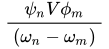
The improved understanding of dynamical systems coming from chaos theory helped shed light on what was termed the small denominator problem or small divisor problem. In the 19th century Poincaré observed (as perhaps had earlier mathematicians) that sometimes 2nd and higher order terms in the perturbative series have "small denominators": That is, they have the general form ${\displaystyle \ {\frac {\ \psi _{n}V\phi _{m}\ }{\ (\omega _{n}-\omega _{m})\ }}\ }$ where ${\displaystyle \ \psi _{n}\ ,}$ ${\displaystyle \ V\ ,}$ and ${\displaystyle \ \phi _{m}\ }$ are some complicated expressions pertinent to the problem to be solved, and ${\displaystyle \ \omega _{n}\ }$ and ${\displaystyle \ \omega _{m}\ }$ are real numbers; very often they are the energy of normal modes. The small divisor problem arises when the difference ${\displaystyle \ \omega _{n}-\omega _{m}\ }$ is small, causing the perturbative correction to "blow up", becoming as large or maybe larger than the zeroth order term. This situation signals a breakdown of perturbation theory: It stops working at this point, and cannot be expanded or summed any further. In formal terms, the perturbative series is an asymptotic series: A useful approximation for a few terms, but at some point becomes less accurate if even more terms are added. The breakthrough from chaos theory was an explanation of why this happened: The small divisors occur whenever perturbation theory is applied to a chaotic system. The one signals the presence of the other.^{[citation needed]}

Since the planets are very remote from each other, and since their mass is small as compared to the mass of the Sun, the gravitational forces between the planets can be neglected, and the planetary motion is considered, to a first approximation, as taking place along Kepler's orbits, which are defined by the equations of the two-body problem, the two bodies being the planet and the Sun.^[14]

Since astronomic data came to be known with much greater accuracy, it became necessary to consider how the motion of a planet around the Sun is affected by other planets. This was the origin of the three-body problem; thus, in studying the system Moon-Earth-Sun, the mass ratio between the Moon and the Earth was chosen as the "small parameter". Lagrange and Laplace were the first to advance the view that the so-called "constants" which describe the motion of a planet around the Sun gradually change: They are "perturbed", as it were, by the motion of other planets and vary as a function of time; hence the name "perturbation theory".^[14]

Perturbation theory was investigated by the classical scholars – Laplace, Siméon Denis Poisson, Carl Friedrich Gauss – as a result of which the computations could be performed with a very high accuracy. The discovery of the planet Neptune in 1848 by Urbain Le Verrier, based on the deviations in motion of the planet Uranus. He sent the coordinates to J.G. Galle who successfully observed Neptune through his telescope – a triumph of perturbation theory.^[14]

The standard exposition of perturbation theory is given in terms of the order to which the perturbation is carried out: first-order perturbation theory or second-order perturbation theory, and whether the perturbed states are degenerate, which requires singular perturbation. In the singular case extra care must be taken, and the theory is slightly more elaborate.