
Trigonometric functions
View on Wikipedia

In mathematics, the trigonometric functions (also called circular functions, angle functions or goniometric functions)[1] are real functions which relate an angle of a right-angled triangle to ratios of two side lengths. They are widely used in all sciences that are related to geometry, such as navigation, solid mechanics, celestial mechanics, geodesy, and many others. They are among the simplest periodic functions, and as such are also widely used for studying periodic phenomena through Fourier analysis.
| Trigonometry |
|---|
 |
| Reference |
| Laws and theorems |
| Calculus |
| Mathematicians |
The trigonometric functions most widely used in modern mathematics are the sine, the cosine, and the tangent functions. Their reciprocals are respectively the cosecant, the secant, and the cotangent functions, which are less used. Each of these six trigonometric functions has a corresponding inverse function and has an analog among the hyperbolic functions.
The oldest definitions of trigonometric functions, related to right-angle triangles, define them only for acute angles. To extend the sine and cosine functions to functions whose domain is the whole real line, geometrical definitions using the standard unit circle (i.e., a circle with radius 1 unit) are often used; then the domain of the other functions is the real line with some isolated points removed. Modern definitions express trigonometric functions as infinite series or as solutions of differential equations. This allows extending the domain of sine and cosine functions to the whole complex plane, and the domain of the other trigonometric functions to the complex plane with some isolated points removed.
Notation
[edit]Conventionally, an abbreviation of each trigonometric function's name is used as its symbol in formulas. Today, the most common versions of these abbreviations are "sin" for sine, "cos" for cosine, "tan" or "tg" for tangent, "sec" for secant, "csc" or "cosec" for cosecant, and "cot" or "ctg" for cotangent. Historically, these abbreviations were first used in prose sentences to indicate particular line segments or their lengths related to an arc of an arbitrary circle, and later to indicate ratios of lengths, but as the function concept developed in the 17th–18th century, they began to be considered as functions of real-number-valued angle measures, and written with functional notation, for example sin(x). Parentheses are still often omitted to reduce clutter, but are sometimes necessary; for example the expression would typically be interpreted to mean so parentheses are required to express


A positive integer appearing as a superscript after the symbol of the function denotes exponentiation, not function composition. For example and denote not This differs from the (historically later) general functional notation in which



In contrast, the superscript is commonly used to denote the inverse function, not the reciprocal. For example and denote the inverse trigonometric function alternatively written The equation implies not In this case, the superscript could be considered as denoting a composed or iterated function, but negative superscripts other than are not in common use.


Right-angled triangle definitions
[edit]

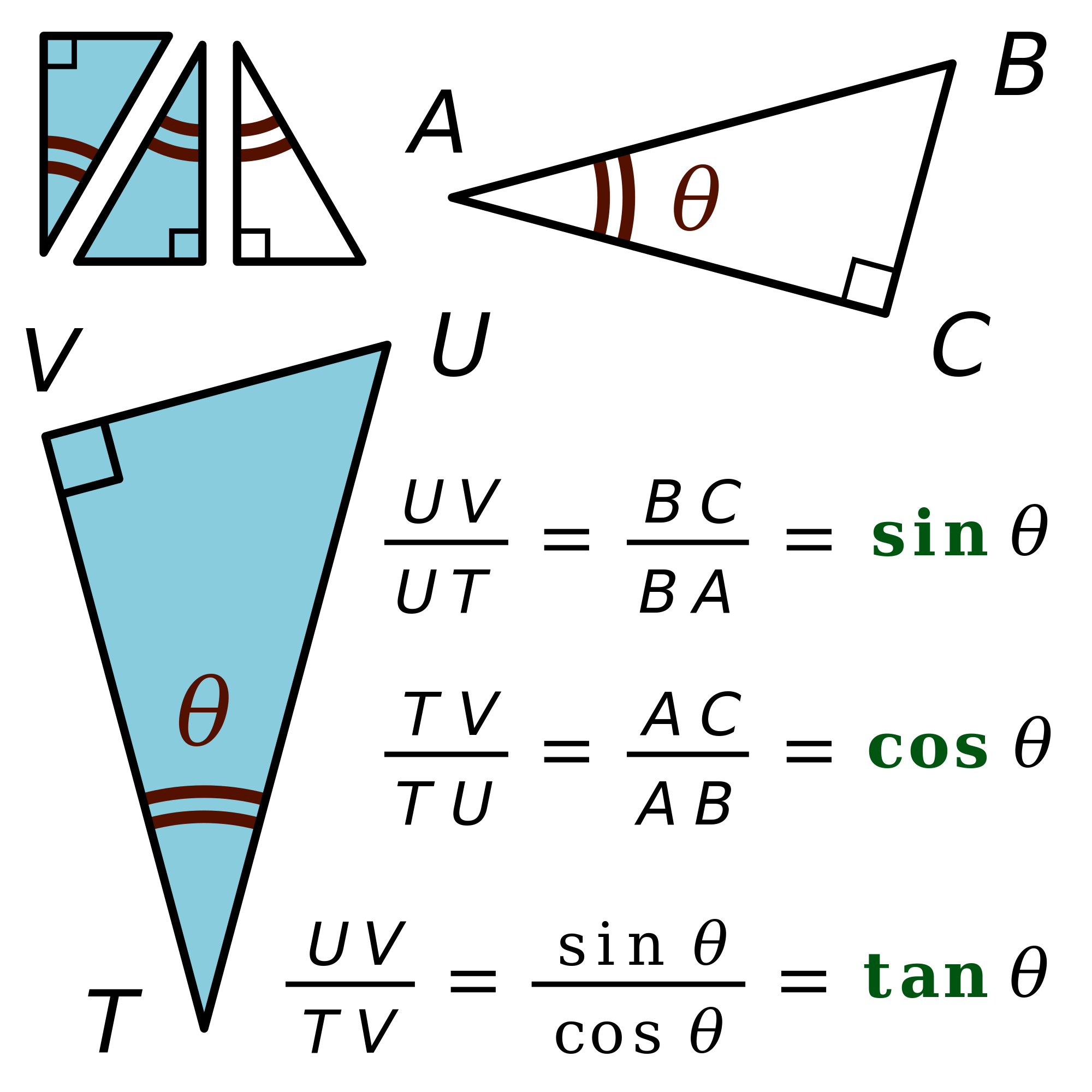
If the acute angle θ is given, then any right triangles that have an angle of θ are similar to each other. This means that the ratio of any two side lengths depends only on θ. Thus these six ratios define six functions of θ, which are the trigonometric functions. In the following definitions, the hypotenuse is the length of the side opposite the right angle, opposite represents the side opposite the given angle θ, and adjacent represents the side between the angle θ and the right angle.[2][3]
|
|
|
|
|
|
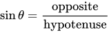
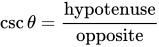
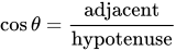
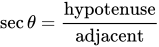
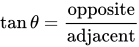
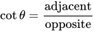
Various mnemonics can be used to remember these definitions.
In a right-angled triangle, the sum of the two acute angles is a right angle, that is, 90° or π/2 radians. Therefore and represent the same ratio, and thus are equal. This identity and analogous relationships between the other trigonometric functions are summarized in the following table.


Bottom: Graph of sine versus angle. Angles from the top panel are identified.
| Function | Description | Relationship | |
|---|---|---|---|
| using radians | using degrees | ||
| sine | opposite/hypotenuse | ||
| cosine | adjacent/hypotenuse | ||
| tangent | opposite/adjacent | ||
| cotangent | adjacent/opposite | ||
| secant | hypotenuse/adjacent | ||
| cosecant | hypotenuse/opposite | ||












Radians versus degrees
[edit]In geometric applications, the argument of a trigonometric function is generally the measure of an angle. For this purpose, any angular unit is convenient. One common unit is degrees, in which a right angle is 90° and a complete turn is 360° (particularly in elementary mathematics).
However, in calculus and mathematical analysis, the trigonometric functions are generally regarded more abstractly as functions of real or complex numbers, rather than angles. In fact, the functions sin and cos can be defined for all complex numbers in terms of the exponential function, via power series,[5] or as solutions to differential equations given particular initial values[6] (see below), without reference to any geometric notions. The other four trigonometric functions (tan, cot, sec, csc) can be defined as quotients and reciprocals of sin and cos, except where zero occurs in the denominator. It can be proved, for real arguments, that these definitions coincide with elementary geometric definitions if the argument is regarded as an angle in radians.[5] Moreover, these definitions result in simple expressions for the derivatives and indefinite integrals for the trigonometric functions.[7] Thus, in settings beyond elementary geometry, radians are regarded as the mathematically natural unit for describing angle measures.
When radians (rad) are employed, the angle is given as the length of the arc of the unit circle subtended by it: the angle that subtends an arc of length 1 on the unit circle is 1 rad (≈ 57.3°),[8] and a complete turn (360°) is an angle of 2π (≈ 6.28) rad.[9] Since radian is dimensionless, i.e. 1 rad = 1, the degree symbol can also be regarded as a mathematical constant factor such that 1° = π/180 ≈ 0.0175.[citation needed]
Unit-circle definitions
[edit]


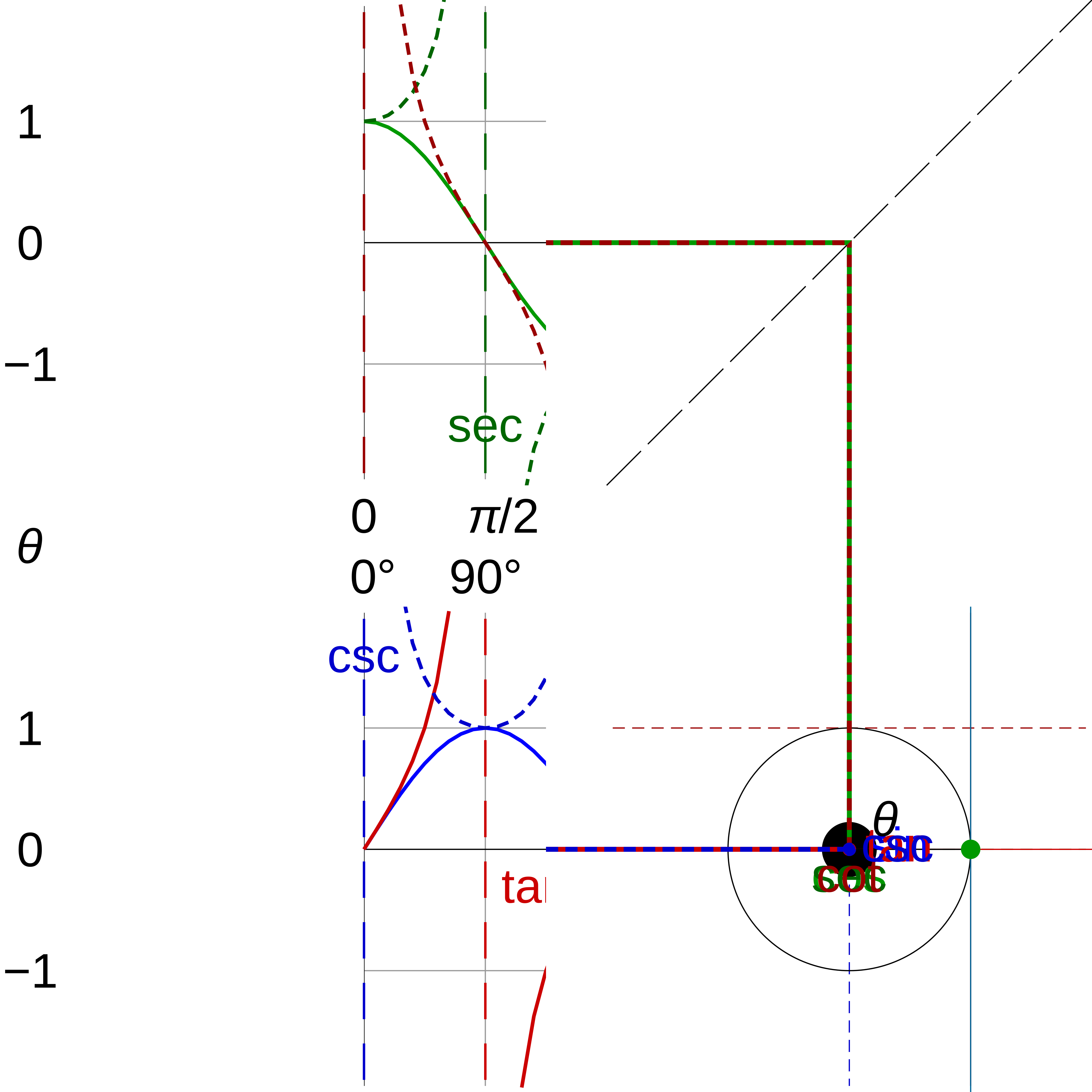
The six trigonometric functions can be defined as coordinate values of points on the Euclidean plane that are related to the unit circle, which is the circle of radius one centered at the origin O of this coordinate system. While right-angled triangle definitions allow for the definition of the trigonometric functions for angles between 0 and radians (90°), the unit circle definitions allow the domain of trigonometric functions to be extended to all positive and negative real numbers.

Let be the ray obtained by rotating by an angle θ the positive half of the x-axis (counterclockwise rotation for and clockwise rotation for ). This ray intersects the unit circle at the point The ray extended to a line if necessary, intersects the line of equation at point and the line of equation at point The tangent line to the unit circle at the point A, is perpendicular to and intersects the y- and x-axes at points and The coordinates of these points give the values of all trigonometric functions for any arbitrary real value of θ in the following manner.


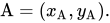


The trigonometric functions cos and sin are defined, respectively, as the x- and y-coordinate values of point A. That is, and [11]


In the range , this definition coincides with the right-angled triangle definition, by taking the right-angled triangle to have the unit radius OA as hypotenuse. And since the equation holds for all points on the unit circle, this definition of cosine and sine also satisfies the Pythagorean identity.



The other trigonometric functions can be found along the unit circle as and and




By applying the Pythagorean identity and geometric proof methods, these definitions can readily be shown to coincide with the definitions of tangent, cotangent, secant and cosecant in terms of sine and cosine, that is


Since a rotation of an angle of does not change the position or size of a shape, the points A, B, C, D, and E are the same for two angles whose difference is an integer multiple of . Thus trigonometric functions are periodic functions with period . That is, the equalities and hold for any angle θ and any integer k. The same is true for the four other trigonometric functions. By observing the sign and the monotonicity of the functions sine, cosine, cosecant, and secant in the four quadrants, one can show that is the smallest value for which they are periodic (i.e., is the fundamental period of these functions). However, after a rotation by an angle , the points B and C already return to their original position, so that the tangent function and the cotangent function have a fundamental period of . That is, the equalities and hold for any angle θ and any integer k.







Algebraic values
[edit]
The algebraic expressions for the most important angles are as follows:
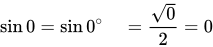
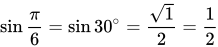
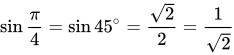
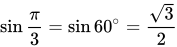
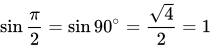
Writing the numerators as square roots of consecutive non-negative integers, with a denominator of 2, provides an easy way to remember the values.[12]
Such simple expressions generally do not exist for other angles which are rational multiples of a right angle.
- For an angle which, measured in degrees, is a multiple of three, the exact trigonometric values of the sine and the cosine may be expressed in terms of square roots. These values of the sine and the cosine may thus be constructed by ruler and compass.
- For an angle of an integer number of degrees, the sine and the cosine may be expressed in terms of square roots and the cube root of a non-real complex number. Galois theory allows a proof that, if the angle is not a multiple of 3°, non-real cube roots are unavoidable.
- For an angle which, expressed in degrees, is a rational number, the sine and the cosine are algebraic numbers, which may be expressed in terms of n-th roots. This results from the fact that the Galois groups of the cyclotomic polynomials are cyclic.
- For an angle which, expressed in degrees, is not a rational number, then either the angle or both the sine and the cosine are transcendental numbers. This is a corollary of Baker's theorem, proved in 1966.
- If the sine of an angle is a rational number then the cosine is not necessarily a rational number, and vice-versa. However if the tangent of an angle is rational then both the sine and cosine of the double angle will be rational.
Simple algebraic values
[edit]The following table lists the sines, cosines, and tangents of multiples of 15 degrees from 0 to 90 degrees.
| Angle, θ, in | ||||
|---|---|---|---|---|
| radians | degrees | |||
| Undefined | ||||


Definitions in analysis
[edit]


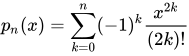
G. H. Hardy noted in his 1908 work A Course of Pure Mathematics that the definition of the trigonometric functions in terms of the unit circle is not satisfactory, because it depends implicitly on a notion of angle that can be measured by a real number.[clarification needed][13] Thus in modern analysis, trigonometric functions are usually constructed without reference to geometry.
Various ways exist in the literature for defining the trigonometric functions in a manner suitable for analysis; they include:
- Using the "geometry" of the unit circle, which requires formulating the arc length of a circle (or area of a sector) analytically.[13]
- By a power series, which is particularly well-suited to complex variables.[13][14]
- By using an infinite product expansion.[13]
- By inverting the inverse trigonometric functions, which can be defined as integrals of algebraic or rational functions.[13]
- As solutions of a differential equation.[15]
Definition by differential equations
[edit]Sine and cosine can be defined as the unique solution to the initial value problem:[16]

Differentiating again, and , so both sine and cosine are solutions of the same ordinary differential equation Sine is the unique solution with y(0) = 0 and y′(0) = 1; cosine is the unique solution with y(0) = 1 and y′(0) = 0.



One can then prove, as a theorem, that solutions are periodic, having the same period. Writing this period as is then a definition of the real number which is independent of geometry.

Applying the quotient rule to the tangent , so the tangent function satisfies the ordinary differential equation It is the unique solution with y(0) = 0.



Power series expansion
[edit]The basic trigonometric functions can be defined by the following power series expansions.[17] These series are also known as the Taylor series or Maclaurin series of these trigonometric functions: The radius of convergence of these series is infinite. Therefore, the sine and the cosine can be extended to entire functions (also called "sine" and "cosine"), which are (by definition) complex-valued functions that are defined and holomorphic on the whole complex plane.
![{\displaystyle {\begin{aligned}\sin x&=x-{\frac {x^{3}}{3!}}+{\frac {x^{5}}{5!}}-{\frac {x^{7}}{7!}}+\cdots \\[6mu]&=\sum _{n=0}^{\infty }{\frac {(-1)^{n}}{(2n+1)!}}x^{2n+1}\\[8pt]\cos x&=1-{\frac {x^{2}}{2!}}+{\frac {x^{4}}{4!}}-{\frac {x^{6}}{6!}}+\cdots \\[6mu]&=\sum _{n=0}^{\infty }{\frac {(-1)^{n}}{(2n)!}}x^{2n}.\end{aligned}}}](https://wikimedia.org/api/rest_v1/media/math/render/svg/396790dc41b52c5381ef1683a279d05ba5d64f79)
Term-by-term differentiation shows that the sine and cosine defined by the series obey the differential equation discussed previously, and conversely one can obtain these series from elementary recursion relations derived from the differential equation.
Being defined as fractions of entire functions, the other trigonometric functions may be extended to meromorphic functions, that is functions that are holomorphic in the whole complex plane, except some isolated points called poles. Here, the poles are the numbers of the form for the tangent and the secant, or for the cotangent and the cosecant, where k is an arbitrary integer.


Recurrences relations may also be computed for the coefficients of the Taylor series of the other trigonometric functions. These series have a finite radius of convergence. Their coefficients have a combinatorial interpretation: they enumerate alternating permutations of finite sets.[18]
More precisely, defining
- Un, the n-th up/down number,
- Bn, the n-th Bernoulli number, and
- En, is the n-th Euler number,
one has the following series expansions:[19]
![{\displaystyle {\begin{aligned}\tan x&{}=\sum _{n=0}^{\infty }{\frac {U_{2n+1}}{(2n+1)!}}x^{2n+1}\\[8mu]&{}=\sum _{n=1}^{\infty }{\frac {(-1)^{n-1}2^{2n}\left(2^{2n}-1\right)B_{2n}}{(2n)!}}x^{2n-1}\\[5mu]&{}=x+{\frac {1}{3}}x^{3}+{\frac {2}{15}}x^{5}+{\frac {17}{315}}x^{7}+\cdots ,\qquad {\text{for }}|x|<{\frac {\pi }{2}}.\end{aligned}}}](https://wikimedia.org/api/rest_v1/media/math/render/svg/d0de1a2399f8c3b723b71c5e24e8f0136fd4bb18)
![{\displaystyle {\begin{aligned}\csc x&=\sum _{n=0}^{\infty }{\frac {(-1)^{n+1}2\left(2^{2n-1}-1\right)B_{2n}}{(2n)!}}x^{2n-1}\\[5mu]&=x^{-1}+{\frac {1}{6}}x+{\frac {7}{360}}x^{3}+{\frac {31}{15120}}x^{5}+\cdots ,\qquad {\text{for }}0<|x|<\pi .\end{aligned}}}](https://wikimedia.org/api/rest_v1/media/math/render/svg/bd4b74fe732906b09b6205ecfa81326222ae0320)
![{\displaystyle {\begin{aligned}\sec x&=\sum _{n=0}^{\infty }{\frac {U_{2n}}{(2n)!}}x^{2n}=\sum _{n=0}^{\infty }{\frac {(-1)^{n}E_{2n}}{(2n)!}}x^{2n}\\[5mu]&=1+{\frac {1}{2}}x^{2}+{\frac {5}{24}}x^{4}+{\frac {61}{720}}x^{6}+\cdots ,\qquad {\text{for }}|x|<{\frac {\pi }{2}}.\end{aligned}}}](https://wikimedia.org/api/rest_v1/media/math/render/svg/1e8d1437d98b6b4d05d4da50fe2e18bd39a7ff9e)
![{\displaystyle {\begin{aligned}\cot x&=\sum _{n=0}^{\infty }{\frac {(-1)^{n}2^{2n}B_{2n}}{(2n)!}}x^{2n-1}\\[5mu]&=x^{-1}-{\frac {1}{3}}x-{\frac {1}{45}}x^{3}-{\frac {2}{945}}x^{5}-\cdots ,\qquad {\text{for }}0<|x|<\pi .\end{aligned}}}](https://wikimedia.org/api/rest_v1/media/math/render/svg/4c6645779d6fe606694a0ac157fcdee271c7e795)
Continued fraction expansion
[edit]The following continued fractions are valid in the whole complex plane:
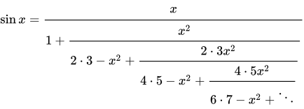
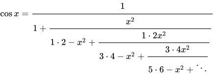
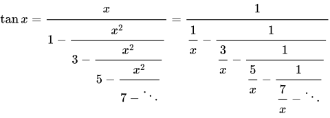
The last one was used in the historically first proof that π is irrational.[20]
Partial fraction expansion
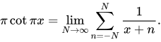
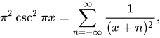
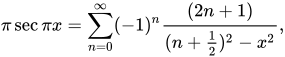
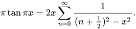
[edit]There is a series representation as partial fraction expansion where just translated reciprocal functions are summed up, such that the poles of the cotangent function and the reciprocal functions match:[21] This identity can be proved with the Herglotz trick.[22] Combining the (–n)-th with the n-th term lead to absolutely convergent series: Similarly, one can find a partial fraction expansion for the secant, cosecant and tangent functions:


Infinite product expansion
[edit]The following infinite product for the sine is due to Leonhard Euler, and is of great importance in complex analysis:[23] This may be obtained from the partial fraction decomposition of given above, which is the logarithmic derivative of .[24] From this, it can be deduced also that




Euler's formula and the exponential function
[edit]

Euler's formula relates sine and cosine to the exponential function: This formula is commonly considered for real values of x, but it remains true for all complex values.

Proof: Let and One has for j = 1, 2. The quotient rule implies thus that . Therefore, is a constant function, which equals 1, as This proves the formula.






One has
![{\displaystyle {\begin{aligned}e^{ix}&=\cos x+i\sin x\\[5pt]e^{-ix}&=\cos x-i\sin x.\end{aligned}}}](https://wikimedia.org/api/rest_v1/media/math/render/svg/8d374fafbe34908c7766b67e4c51797589906940)
Solving this linear system in sine and cosine, one can express them in terms of the exponential function:
![{\displaystyle {\begin{aligned}\sin x&={\frac {e^{ix}-e^{-ix}}{2i}}\\[5pt]\cos x&={\frac {e^{ix}+e^{-ix}}{2}}.\end{aligned}}}](https://wikimedia.org/api/rest_v1/media/math/render/svg/590e4a1bbe3ccdb7521fe06a6e5b56e538d4e729)
When x is real, this may be rewritten as

Most trigonometric identities can be proved by expressing trigonometric functions in terms of the complex exponential function by using above formulas, and then using the identity for simplifying the result.

Euler's formula can also be used to define the basic trigonometric function directly, as follows, using the language of topological groups.[25] The set of complex numbers of unit modulus is a compact and connected topological group, which has a neighborhood of the identity that is homeomorphic to the real line. Therefore, it is isomorphic as a topological group to the one-dimensional torus group , via an isomorphism In simple terms, , and this isomorphism is unique up to taking complex conjugates.


For a nonzero real number (the base), the function defines an isomorphism of the group . The real and imaginary parts of are the cosine and sine, where is used as the base for measuring angles. For example, when , we get the measure in radians, and the usual trigonometric functions. When , we get the sine and cosine of angles measured in degrees.


Note that is the unique value at which the derivative becomes a unit vector with positive imaginary part at . This fact can, in turn, be used to define the constant .


Definition via integration
[edit]Another way to define the trigonometric functions in analysis is using integration.[13][26] For a real number , put where this defines this inverse tangent function. Also, is defined by a definition that goes back to Karl Weierstrass.[27]


On the interval , the trigonometric functions are defined by inverting the relation . Thus we define the trigonometric functions by where the point is on the graph of and the positive square root is taken.



This defines the trigonometric functions on . The definition can be extended to all real numbers by first observing that, as , , and so and . Thus and are extended continuously so that . Now the conditions and define the sine and cosine as periodic functions with period , for all real numbers.


Proving the basic properties of sine and cosine, including the fact that sine and cosine are analytic, one may first establish the addition formulae. First, holds, provided , since after the substitution . In particular, the limiting case as gives Thus we have and So the sine and cosine functions are related by translation over a quarter period .


Definitions using functional equations
[edit]One can also define the trigonometric functions using various functional equations.
For example,[28] the sine and the cosine form the unique pair of continuous functions that satisfy the difference formula and the added condition


In the complex plane
[edit]The sine and cosine of a complex number can be expressed in terms of real sines, cosines, and hyperbolic functions as follows:

![{\displaystyle {\begin{aligned}\sin z&=\sin x\cosh y+i\cos x\sinh y\\[5pt]\cos z&=\cos x\cosh y-i\sin x\sinh y\end{aligned}}}](https://wikimedia.org/api/rest_v1/media/math/render/svg/c1646655eab602e234f42df85cae241ffbb867cf)
By taking advantage of domain coloring, it is possible to graph the trigonometric functions as complex-valued functions. Various features unique to the complex functions can be seen from the graph; for example, the sine and cosine functions can be seen to be unbounded as the imaginary part of becomes larger (since the color white represents infinity), and the fact that the functions contain simple zeros or poles is apparent from the fact that the hue cycles around each zero or pole exactly once. Comparing these graphs with those of the corresponding Hyperbolic functions highlights the relationships between the two.


|


|


|


Periodicity and asymptotes
[edit]The sine and cosine functions are periodic, with period , which is the smallest positive period: Consequently, the cosecant and secant also have as their period.

The functions sine and cosine also have semiperiods , and and consequently Also, (see Complementary angles).


The function has a unique zero (at ) in the strip . The function has the pair of zeros in the same strip. Because of the periodicity, the zeros of sine are There zeros of cosine are All of the zeros are simple zeros, and both functions have derivative at each of the zeros.


The tangent function has a simple zero at and vertical asymptotes at , where it has a simple pole of residue . Again, owing to the periodicity, the zeros are all the integer multiples of and the poles are odd multiples of , all having the same residue. The poles correspond to vertical asymptotes


The cotangent function has a simple pole of residue 1 at the integer multiples of and simple zeros at odd multiples of . The poles correspond to vertical asymptotes


Basic identities
[edit]Many identities interrelate the trigonometric functions. This section contains the most basic ones; for more identities, see List of trigonometric identities. These identities may be proved geometrically from the unit-circle definitions or the right-angled-triangle definitions (although, for the latter definitions, care must be taken for angles that are not in the interval [0, π/2], see Proofs of trigonometric identities). For non-geometrical proofs using only tools of calculus, one may use directly the differential equations, in a way that is similar to that of the above proof of Euler's identity. One can also use Euler's identity for expressing all trigonometric functions in terms of complex exponentials and using properties of the exponential function.
Parity
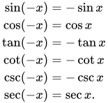
[edit]The cosine and the secant are even functions; the other trigonometric functions are odd functions. That is:
Periods
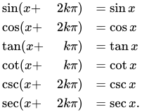
[edit]All trigonometric functions are periodic functions of period 2π. This is the smallest period, except for the tangent and the cotangent, which have π as smallest period. This means that, for every integer k, one has See Periodicity and asymptotes.
Pythagorean identity
[edit]The Pythagorean identity, is the expression of the Pythagorean theorem in terms of trigonometric functions. It is . Dividing through by either or gives and .





Sum and difference formulas
[edit]The sum and difference formulas allow expanding the sine, the cosine, and the tangent of a sum or a difference of two angles in terms of sines and cosines and tangents of the angles themselves. These can be derived geometrically, using arguments that date to Ptolemy (see Angle sum and difference identities). One can also produce them algebraically using Euler's formula.
- Sum
![{\displaystyle {\begin{aligned}\sin \left(x+y\right)&=\sin x\cos y+\cos x\sin y,\\[5mu]\cos \left(x+y\right)&=\cos x\cos y-\sin x\sin y,\\[5mu]\tan(x+y)&={\frac {\tan x+\tan y}{1-\tan x\tan y}}.\end{aligned}}}](https://wikimedia.org/api/rest_v1/media/math/render/svg/7a94648d4600a711a8851dfaea622a269be4eda5)
- Difference
![{\displaystyle {\begin{aligned}\sin \left(x-y\right)&=\sin x\cos y-\cos x\sin y,\\[5mu]\cos \left(x-y\right)&=\cos x\cos y+\sin x\sin y,\\[5mu]\tan(x-y)&={\frac {\tan x-\tan y}{1+\tan x\tan y}}.\end{aligned}}}](https://wikimedia.org/api/rest_v1/media/math/render/svg/0a627a03bba700c34bee8de20cfa09d78b127716)
When the two angles are equal, the sum formulas reduce to simpler equations known as the double-angle formulae.
![{\displaystyle {\begin{aligned}\sin 2x&=2\sin x\cos x={\frac {2\tan x}{1+\tan ^{2}x}},\\[5mu]\cos 2x&=\cos ^{2}x-\sin ^{2}x=2\cos ^{2}x-1=1-2\sin ^{2}x={\frac {1-\tan ^{2}x}{1+\tan ^{2}x}},\\[5mu]\tan 2x&={\frac {2\tan x}{1-\tan ^{2}x}}.\end{aligned}}}](https://wikimedia.org/api/rest_v1/media/math/render/svg/d631768e76acdd703625fbcaf9cdf8b8e3e9200f)
These identities can be used to derive the product-to-sum identities.
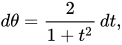
By setting (see half-angle formulae), all trigonometric functions of can be expressed as rational fractions of : Together with this is the tangent half-angle substitution, which reduces the computation of integrals and antiderivatives of trigonometric functions to that of rational fractions.


![{\displaystyle {\begin{aligned}\sin \theta &={\frac {2t}{1+t^{2}}},\\[5mu]\cos \theta &={\frac {1-t^{2}}{1+t^{2}}},\\[5mu]\tan \theta &={\frac {2t}{1-t^{2}}}.\end{aligned}}}](https://wikimedia.org/api/rest_v1/media/math/render/svg/c9eb5a515edf456acce4c943b43121632bef4d27)
Derivatives and antiderivatives
[edit]The derivatives of trigonometric functions result from those of sine and cosine by applying the quotient rule. The values given for the antiderivatives in the following table can be verified by differentiating them. The number C is a constant of integration.








Note: For the integral of can also be written as and the integral of for as where is the inverse hyperbolic sine.



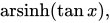

Alternatively, the derivatives of the 'co-functions' can be obtained using trigonometric identities and the chain rule:

Inverse functions
[edit]The trigonometric functions are periodic, and hence not injective, so strictly speaking, they do not have an inverse function. However, on each interval on which a trigonometric function is monotonic, one can define an inverse function, and this defines inverse trigonometric functions as multivalued functions. To define a true inverse function, one must restrict the domain to an interval where the function is monotonic, and is thus bijective from this interval to its image by the function. The common choice for this interval, called the set of principal values, is given in the following table. As usual, the inverse trigonometric functions are denoted with the prefix "arc" before the name or its abbreviation of the function.
| Function | Definition | Domain | Set of principal values |
|---|---|---|---|


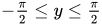



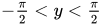







The notations sin−1, cos−1, etc. are often used for arcsin and arccos, etc. When this notation is used, inverse functions could be confused with multiplicative inverses. The notation with the "arc" prefix avoids such a confusion, though "arcsec" for arcsecant can be confused with "arcsecond".
Just like the sine and cosine, the inverse trigonometric functions can also be expressed in terms of infinite series. They can also be expressed in terms of complex logarithms.
Applications
[edit]Angles and sides of a triangle
[edit]In this section A, B, C denote the three (interior) angles of a triangle, and a, b, c denote the lengths of the respective opposite edges. They are related by various formulas, which are named by the trigonometric functions they involve.
Law of sines
[edit]The law of sines states that for an arbitrary triangle with sides a, b, and c and angles opposite those sides A, B and C: where Δ is the area of the triangle, or, equivalently, where R is the triangle's circumradius.


It can be proved by dividing the triangle into two right ones and using the above definition of sine. The law of sines is useful for computing the lengths of the unknown sides in a triangle if two angles and one side are known. This is a common situation occurring in triangulation, a technique to determine unknown distances by measuring two angles and an accessible enclosed distance.
Law of cosines
[edit]The law of cosines (also known as the cosine formula or cosine rule) is an extension of the Pythagorean theorem: or equivalently,

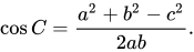
In this formula the angle at C is opposite to the side c. This theorem can be proved by dividing the triangle into two right ones and using the Pythagorean theorem.
The law of cosines can be used to determine a side of a triangle if two sides and the angle between them are known. It can also be used to find the cosines of an angle (and consequently the angles themselves) if the lengths of all the sides are known.
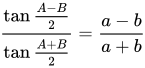
Law of tangents
[edit]The law of tangents says that: .
Law of cotangents
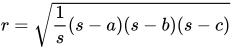
[edit]If s is the triangle's semiperimeter, (a + b + c)/2, and r is the radius of the triangle's incircle, then rs is the triangle's area. Therefore Heron's formula implies that:
.
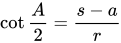
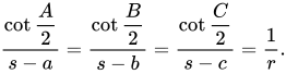
The law of cotangents says that:[29] It follows that
Periodic functions
[edit]


The trigonometric functions are also important in physics. The sine and the cosine functions, for example, are used to describe simple harmonic motion, which models many natural phenomena, such as the movement of a mass attached to a spring and, for small angles, the pendular motion of a mass hanging by a string. The sine and cosine functions are one-dimensional projections of uniform circular motion.
Trigonometric functions also prove to be useful in the study of general periodic functions. The characteristic wave patterns of periodic functions are useful for modeling recurring phenomena such as sound or light waves.[30]
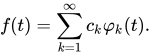
Under rather general conditions, a periodic function f (x) can be expressed as a sum of sine waves or cosine waves in a Fourier series.[31] Denoting the sine or cosine basis functions by φk, the expansion of the periodic function f (t) takes the form:
For example, the square wave can be written as the Fourier series
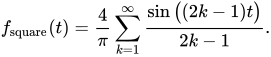
In the animation of a square wave at top right it can be seen that just a few terms already produce a fairly good approximation. The superposition of several terms in the expansion of a sawtooth wave are shown underneath.
History
[edit]While the early study of trigonometry can be traced to antiquity, the trigonometric functions as they are in use today were developed in the medieval period. The chord function was defined by Hipparchus of Nicaea (180–125 BCE) and Ptolemy of Roman Egypt (90–165 CE). The functions of sine and versine (1 − cosine) are closely related to the jyā and koti-jyā functions used in Gupta period Indian astronomy (Aryabhatiya, Surya Siddhanta), via translation from Sanskrit to Arabic and then from Arabic to Latin.[32] (See Aryabhata's sine table.)
All six trigonometric functions in current use were known in Islamic mathematics by the 9th century, as was the law of sines, used in solving triangles.[33] Al-Khwārizmī (c. 780–850) produced tables of sines and cosines. Circa 860, Habash al-Hasib al-Marwazi defined the tangent and the cotangent, and produced their tables.[34][35] Muhammad ibn Jābir al-Harrānī al-Battānī (853–929) defined the reciprocal functions of secant and cosecant, and produced the first table of cosecants for each degree from 1° to 90°.[35] The trigonometric functions were later studied by mathematicians including Omar Khayyám, Bhāskara II, Nasir al-Din al-Tusi, Jamshīd al-Kāshī (14th century), Ulugh Beg (14th century), Regiomontanus (1464), Rheticus, and Rheticus' student Valentinus Otho.
Madhava of Sangamagrama (c. 1400) made early strides in the analysis of trigonometric functions in terms of infinite series.[36] (See Madhava series and Madhava's sine table.)
The tangent function was brought to Europe by Giovanni Bianchini in 1467 in trigonometry tables he created to support the calculation of stellar coordinates.[37]
The terms tangent and secant were first introduced by the Danish mathematician Thomas Fincke in his book Geometria rotundi (1583).[38]
The 17th century French mathematician Albert Girard made the first published use of the abbreviations sin, cos, and tan in his book Trigonométrie.[39]
In a paper published in 1682, Gottfried Leibniz proved that sin x is not an algebraic function of x.[40] Though defined as ratios of sides of a right triangle, and thus appearing to be rational functions, Leibnitz result established that they are actually transcendental functions of their argument. The task of assimilating circular functions into algebraic expressions was accomplished by Euler in his Introduction to the Analysis of the Infinite (1748). His method was to show that the sine and cosine functions are alternating series formed from the even and odd terms respectively of the exponential series. He presented "Euler's formula", as well as near-modern abbreviations (sin., cos., tang., cot., sec., and cosec.).[32]
A few functions were common historically, but are now seldom used, such as the chord, versine (which appeared in the earliest tables[32]), haversine, coversine,[41] half-tangent (tangent of half an angle), and exsecant. List of trigonometric identities shows more relations between these functions.
![{\displaystyle {\begin{aligned}\operatorname {crd} \theta &=2\sin {\tfrac {1}{2}}\theta ,\\[5mu]\operatorname {vers} \theta &=1-\cos \theta =2\sin ^{2}{\tfrac {1}{2}}\theta ,\\[5mu]\operatorname {hav} \theta &={\tfrac {1}{2}}\operatorname {vers} \theta =\sin ^{2}{\tfrac {1}{2}}\theta ,\\[5mu]\operatorname {covers} \theta &=1-\sin \theta =\operatorname {vers} {\bigl (}{\tfrac {1}{2}}\pi -\theta {\bigr )},\\[5mu]\operatorname {exsec} \theta &=\sec \theta -1.\end{aligned}}}](https://wikimedia.org/api/rest_v1/media/math/render/svg/86a41622d234c91baba564f48637953db4bfe0d6)
Historically, trigonometric functions were often combined with logarithms in compound functions like the logarithmic sine, logarithmic cosine, logarithmic secant, logarithmic cosecant, logarithmic tangent and logarithmic cotangent.[42][43][44][45]
Etymology
[edit]The word sine derives[46] from Latin sinus, meaning "bend; bay", and more specifically "the hanging fold of the upper part of a toga", "the bosom of a garment", which was chosen as the translation of what was interpreted as the Arabic word jaib, meaning "pocket" or "fold" in the twelfth-century translations of works by Al-Battani and al-Khwārizmī into Medieval Latin.[47] The choice was based on a misreading of the Arabic written form j-y-b (جيب), which itself originated as a transliteration from Sanskrit jīvā, which along with its synonym jyā (the standard Sanskrit term for the sine) translates to "bowstring", being in turn adopted from Ancient Greek χορδή "string".[48]
The word tangent comes from Latin tangens meaning "touching", since the line touches the circle of unit radius, whereas secant stems from Latin secans—"cutting"—since the line cuts the circle.[49]
The prefix "co-" (in "cosine", "cotangent", "cosecant") is found in Edmund Gunter's Canon triangulorum (1620), which defines the cosinus as an abbreviation of the sinus complementi (sine of the complementary angle) and proceeds to define the cotangens similarly.[50][51]
See also
[edit]Notes
[edit]- ^ Klein, Felix (1924) [1902]. "Die goniometrischen Funktionen". Elementarmathematik vom höheren Standpunkt aus: Arithmetik, Algebra, Analysis (in German). Vol. 1 (3rd ed.). Berlin: J. Springer. Ch. 3.2, p. 175 ff. Translated as "The Goniometric Functions". Elementary Mathematics from an Advanced Standpoint: Arithmetic, Algebra, Analysis. Translated by Hedrick, E. R.; Noble, C. A. Macmillan. 1932. Ch. 3.2, p. 162 ff.
- ^ Protter & Morrey (1970, pp. APP-2, APP-3)
- ^ "Sine, Cosine, Tangent". www.mathsisfun.com. Retrieved 2020-08-29.
- ^ Protter & Morrey (1970, p. APP-7)
- ^ a b Rudin, Walter, 1921–2010. Principles of mathematical analysis (Third ed.). New York. ISBN 0-07-054235-X. OCLC 1502474.
{{cite book}}: CS1 maint: multiple names: authors list (link) CS1 maint: numeric names: authors list (link) - ^ Diamond, Harvey (2014). "Defining Exponential and Trigonometric Functions Using Differential Equations". Mathematics Magazine. 87 (1): 37–42. doi:10.4169/math.mag.87.1.37. ISSN 0025-570X. S2CID 126217060.
- ^ Spivak, Michael (1967). "15". Calculus. Addison-Wesley. pp. 256–257. LCCN 67-20770.
- ^ Sloane, N. J. A. (ed.). "Sequence A072097 (Decimal expansion of 180/Pi)". The On-Line Encyclopedia of Integer Sequences. OEIS Foundation.
- ^ Sloane, N. J. A. (ed.). "Sequence A019692 (Decimal expansion of 2*Pi)". The On-Line Encyclopedia of Integer Sequences. OEIS Foundation.
- ^ Stueben, Michael; Sandford, Diane (1998). Twenty years before the blackboard: the lessons and humor of a mathematics teacher. Spectrum series. Washington, DC: Mathematical Association of America. p. 119. ISBN 978-0-88385-525-6.
- ^ Bityutskov, V.I. (2011-02-07). "Trigonometric Functions". Encyclopedia of Mathematics. Archived from the original on 2017-12-29. Retrieved 2017-12-29.
- ^ Larson, Ron (2013). Trigonometry (9th ed.). Cengage Learning. p. 153. ISBN 978-1-285-60718-4. Archived from the original on 2018-02-15. Extract of page 153 Archived 15 February 2018 at the Wayback Machine
- ^ a b c d e f Hardy, G.H. (1950), A course of pure mathematics (8th ed.), pp. 432–438
- ^ Whittaker, E. T., & Watson, G. N. (1920). A course of modern analysis: an introduction to the general theory of infinite processes and of analytic functions; with an account of the principal transcendental functions. University press.
- ^ Bartle, R. G., & Sherbert, D. R. (2000). Introduction to real analysis (3rd ed). Wiley.
- ^ Bartle & Sherbert 1999, p. 247.
- ^ Whitaker and Watson, p 584
- ^ Stanley, Enumerative Combinatorics, Vol I., p. 149
- ^ Abramowitz; Weisstein.
- ^ Lambert, Johann Heinrich (2004) [1768], "Mémoire sur quelques propriétés remarquables des quantités transcendantes circulaires et logarithmiques", in Berggren, Lennart; Borwein, Jonathan M.; Borwein, Peter B. (eds.), Pi, a source book (3rd ed.), New York: Springer-Verlag, pp. 129–140, ISBN 0-387-20571-3
- ^ Aigner, Martin; Ziegler, Günter M. (2000). Proofs from THE BOOK (Second ed.). Springer-Verlag. p. 149. ISBN 978-3-642-00855-9. Archived from the original on 2014-03-08.
- ^ Remmert, Reinhold (1991). Theory of complex functions. Springer. p. 327. ISBN 978-0-387-97195-7. Archived from the original on 2015-03-20. Extract of page 327 Archived 20 March 2015 at the Wayback Machine
- ^ Whittaker and Watson, p 137
- ^ Ahlfors, p 197
- ^ Bourbaki, Nicolas (1981). Topologie generale. Springer. §VIII.2.
- ^ Bartle (1964), Elements of real analysis, pp. 315–316
- ^ Weierstrass, Karl (1841). "Darstellung einer analytischen Function einer complexen Veränderlichen, deren absoluter Betrag zwischen zwei gegebenen Grenzen liegt" [Representation of an analytical function of a complex variable, whose absolute value lies between two given limits]. Mathematische Werke (in German). Vol. 1. Berlin: Mayer & Müller (published 1894). pp. 51–66.
- ^ Kannappan, Palaniappan (2009). Functional Equations and Inequalities with Applications. Springer. ISBN 978-0387894911.
- ^ The Universal Encyclopaedia of Mathematics, Pan Reference Books, 1976, pp. 529–530. English version George Allen and Unwin, 1964. Translated from the German version Meyers Rechenduden, 1960.
- ^ Farlow, Stanley J. (1993). Partial differential equations for scientists and engineers (Reprint of Wiley 1982 ed.). Courier Dover Publications. p. 82. ISBN 978-0-486-67620-3. Archived from the original on 2015-03-20.
- ^ See for example, Folland, Gerald B. (2009). "Convergence and completeness". Fourier Analysis and its Applications (Reprint of Wadsworth & Brooks/Cole 1992 ed.). American Mathematical Society. pp. 77ff. ISBN 978-0-8218-4790-9. Archived from the original on 2015-03-19.
- ^ a b c Boyer, Carl B. (1991). A History of Mathematics (Second ed.). John Wiley & Sons, Inc. ISBN 0-471-54397-7, p. 210.
- ^ Gingerich, Owen (1986). "Islamic Astronomy". Scientific American. Vol. 254. p. 74. Archived from the original on 2013-10-19. Retrieved 2010-07-13.
- ^ Jacques Sesiano, "Islamic mathematics", p. 157, in Selin, Helaine; D'Ambrosio, Ubiratan, eds. (2000). Mathematics Across Cultures: The History of Non-western Mathematics. Springer Science+Business Media. ISBN 978-1-4020-0260-1.
- ^ a b "trigonometry". Encyclopedia Britannica. 2023-11-17.
- ^ O'Connor, J. J.; Robertson, E. F. "Madhava of Sangamagrama". School of Mathematics and Statistics University of St Andrews, Scotland. Archived from the original on 2006-05-14. Retrieved 2007-09-08.
- ^ Van Brummelen, Glen (2018). "The end of an error: Bianchini, Regiomontanus, and the tabulation of stellar coordinates". Archive for History of Exact Sciences. 72 (5): 547–563. doi:10.1007/s00407-018-0214-2. JSTOR 45211959. S2CID 240294796.
- ^ "Fincke biography". Archived from the original on 2017-01-07. Retrieved 2017-03-15.
- ^ O'Connor, John J.; Robertson, Edmund F., "Trigonometric functions", MacTutor History of Mathematics Archive, University of St Andrews
- ^ Bourbaki, Nicolás (1994). Elements of the History of Mathematics. Springer. ISBN 9783540647676.
- ^ Nielsen (1966, pp. xxiii–xxiv)
- ^ von Hammer, Ernst Hermann Heinrich [in German], ed. (1897). Lehrbuch der ebenen und sphärischen Trigonometrie. Zum Gebrauch bei Selbstunterricht und in Schulen, besonders als Vorbereitung auf Geodäsie und sphärische Astronomie (in German) (2 ed.). Stuttgart, Germany: J. B. Metzlerscher Verlag. Retrieved 2024-02-06.
- ^ Heß, Adolf (1926) [1916]. Trigonometrie für Maschinenbauer und Elektrotechniker - Ein Lehr- und Aufgabenbuch für den Unterricht und zum Selbststudium (in German) (6 ed.). Winterthur, Switzerland: Springer. doi:10.1007/978-3-662-36585-4. ISBN 978-3-662-35755-2.
{{cite book}}: ISBN / Date incompatibility (help) - ^ Lötzbeyer, Philipp (1950). "§ 14. Erläuterungen u. Beispiele zu T. 13: lg sin X; lg cos X und T. 14: lg tg x; lg ctg X". Erläuterungen und Beispiele für den Gebrauch der vierstelligen Tafeln zum praktischen Rechnen (in German) (1 ed.). Berlin, Germany: Walter de Gruyter & Co. doi:10.1515/9783111507545. ISBN 978-3-11114038-4. Archive ID 541650. Retrieved 2024-02-06.
{{cite book}}: ISBN / Date incompatibility (help) - ^ Roegel, Denis, ed. (2016-08-30). A reconstruction of Peters's table of 7-place logarithms (volume 2, 1940). Vandoeuvre-lès-Nancy, France: Université de Lorraine. hal-01357842. Archived from the original on 2024-02-06. Retrieved 2024-02-06.
- ^ The anglicized form is first recorded in 1593 in Thomas Fale's Horologiographia, the Art of Dialling.
- ^ Various sources credit the first use of sinus to either
- Plato Tiburtinus's 1116 translation of the Astronomy of Al-Battani
- Gerard of Cremona's translation of the Algebra of al-Khwārizmī
- Robert of Chester's 1145 translation of the tables of al-Khwārizmī
See Maor (1998), chapter 3, for an earlier etymology crediting Gerard.
See Katx, Victor (July 2008). A history of mathematics (3rd ed.). Boston: Pearson. p. 210 (sidebar). ISBN 978-0321387004. - ^ See Plofker, Mathematics in India, Princeton University Press, 2009, p. 257
See "Clark University". Archived from the original on 2008-06-15.
See Maor (1998), chapter 3, regarding the etymology. - ^ Oxford English Dictionary
- ^ Gunter, Edmund (1620). Canon triangulorum.
- ^ Roegel, Denis, ed. (2010-12-06). "A reconstruction of Gunter's Canon triangulorum (1620)" (Research report). HAL. inria-00543938. Archived from the original on 2017-07-28. Retrieved 2017-07-28.
References
[edit]- Abramowitz, Milton; Stegun, Irene Ann, eds. (1983) [June 1964]. Handbook of Mathematical Functions with Formulas, Graphs, and Mathematical Tables. Applied Mathematics Series. Vol. 55 (Ninth reprint with additional corrections of tenth original printing with corrections (December 1972); first ed.). Washington D.C.; New York: United States Department of Commerce, National Bureau of Standards; Dover Publications. ISBN 978-0-486-61272-0. LCCN 64-60036. MR 0167642. LCCN 65-12253.
- Lars Ahlfors, Complex Analysis: an introduction to the theory of analytic functions of one complex variable, second edition, McGraw-Hill Book Company, New York, 1966.
- Bartle, Robert G.; Sherbert, Donald R. (1999). Introduction to Real Analysis (3rd ed.). Wiley. ISBN 9780471321484.
- Boyer, Carl B., A History of Mathematics, John Wiley & Sons, Inc., 2nd edition. (1991). ISBN 0-471-54397-7.
- Cajori, Florian (1929). "§2.2.1. Trigonometric Notations". A History of Mathematical Notations. Vol. 2. Open Court. pp. 142–179 (¶511–537).
- Gal, Shmuel and Bachelis, Boris. An accurate elementary mathematical library for the IEEE floating point standard, ACM Transactions on Mathematical Software (1991).
- Joseph, George G., The Crest of the Peacock: Non-European Roots of Mathematics, 2nd ed. Penguin Books, London. (2000). ISBN 0-691-00659-8.
- Kantabutra, Vitit, "On hardware for computing exponential and trigonometric functions," IEEE Trans. Computers 45 (3), 328–339 (1996).
- Maor, Eli, Trigonometric Delights, Princeton Univ. Press. (1998). Reprint edition (2002): ISBN 0-691-09541-8.
- Needham, Tristan, "Preface"" to Visual Complex Analysis. Oxford University Press, (1999). ISBN 0-19-853446-9.
- Nielsen, Kaj L. (1966), Logarithmic and Trigonometric Tables to Five Places (2nd ed.), New York: Barnes & Noble, LCCN 61-9103
- O'Connor, J. J., and E. F. Robertson, "Trigonometric functions", MacTutor History of Mathematics archive. (1996).
- O'Connor, J. J., and E. F. Robertson, "Madhava of Sangamagramma", MacTutor History of Mathematics archive. (2000).
- Pearce, Ian G., "Madhava of Sangamagramma" Archived 2006-05-05 at the Wayback Machine, MacTutor History of Mathematics archive. (2002).
- Protter, Murray H.; Morrey, Charles B. Jr. (1970), College Calculus with Analytic Geometry (2nd ed.), Reading: Addison-Wesley, LCCN 76087042
- Weisstein, Eric W., "Tangent" from MathWorld, accessed 21 January 2006.
External links
[edit]
- "Trigonometric functions", Encyclopedia of Mathematics, EMS Press, 2001 [1994]
- Visionlearning Module on Wave Mathematics
- GonioLab Visualization of the unit circle, trigonometric and hyperbolic functions
- q-Sine Article about the q-analog of sin at MathWorld
- q-Cosine Article about the q-analog of cos at MathWorld
| International | |
|---|---|
| National | |
| Other | |

Trigonometric functions
View on GrokipediaIntroductory Concepts
Notation
The primary trigonometric functions are denoted using the following standard symbols: sine by , cosine by , tangent by , cotangent by , secant by , and cosecant by . These abbreviations, shortened from their full names (such as "sine" from Latin sinus and "tangent" from the geometric line), have become the conventional notation in mathematical texts since the 17th century. The reciprocal relationships are implicit in the notation, with as the reciprocal of , of , and of .[6] Historically, trigonometric notation evolved from earlier forms using full words or alternative abbreviations, such as "S" for sine or "R" for the radius in chord-based computations, to the more compact modern symbols introduced in the 1600s. For instance, the abbreviations "sin" and "cos" were introduced by Edmund Gunter around 1620–1624, while "tan" dates to Thomas Fincke's 1583 text; Gottfried Wilhelm Leibniz further popularized functional notation like in the late 17th century, treating these as functions of a variable rather than fixed ratios.[7] This shift from verbose or geometric-specific symbols to concise, function-oriented ones facilitated the integration of trigonometry into calculus and analysis.[3] The argument of a trigonometric function, which represents the input angle or value, is typically denoted by (theta) in geometric and introductory contexts to highlight its angular interpretation, often in conjunction with units like degrees or radians. In contrast, is the standard variable for arguments in broader mathematical applications, including real or complex numbers, allowing trigonometric functions to be analyzed as part of general function theory.[8] Multi-angle notations, such as or where is an integer, extend the basic function symbols to express compositions or multiples of the argument, enabling compact representation of periodic extensions and laying the groundwork for exploring relationships among trigonometric values.[9] These forms underscore the functions' versatility in modeling oscillations and waves without altering the core symbolic conventions.Angle Measurement
Angles are measured using two primary units: degrees and radians. The degree, denoted by the symbol °, is defined such that one complete rotation around a circle corresponds to 360 degrees. This unit traces its origins to ancient Babylonian astronomy, where the sexagesimal (base-60) system led to the division of the full circle—or the ecliptic path of the sun—into 360 equal parts for tracking celestial movements.[10][11] In contrast, the radian provides a more geometrically natural measure of angles. One radian is the central angle subtended at the center of a circle by an arc whose length equals the circle's radius. Consequently, a full rotation around the circle measures exactly radians, linking angular measure directly to the circle's circumference. To convert between these units, the formula radians = degrees is used, reflecting the proportional relationship between the two systems. This conversion is essential for applications spanning geometry and analysis. Radians hold particular advantages in calculus, where trigonometric functions are differentiated and integrated. For instance, the derivative of is precisely when is measured in radians, avoiding extraneous scaling factors that arise with degrees. This property simplifies many analytical computations and aligns angular measures with linear dimensions in a unit circle.[12]Right Triangle Definitions
The trigonometric functions can be defined geometrically using the ratios of the sides of a right-angled triangle, where one angle is exactly 90° and the other two angles are acute. In such a triangle, the side opposite the right angle is called the hypotenuse, which is the longest side, while the other two sides are the legs: one adjacent to the acute angle of interest and the other opposite to it.[13][14] Consider an acute angle in a right triangle, with the opposite side of length , the adjacent side of length , and the hypotenuse of length . The sine function is defined as the ratio of the opposite side to the hypotenuse: . The cosine function is the ratio of the adjacent side to the hypotenuse: . The tangent function is the ratio of the opposite side to the adjacent side: .[13][14] The remaining three trigonometric functions are the reciprocals of these: the cosecant is , the secant is , and the cotangent is . These definitions apply specifically to acute angles in the right triangle, so (or in radians), where all ratios are positive.[13][14] To visualize, imagine a right triangle with the right angle at vertex C, acute angle at vertex A, opposite side (from B to C), adjacent side (from A to C), and hypotenuse (from A to B); the labels align with the standard ratios above. A common mnemonic for recalling the definitions of sine, cosine, and tangent is SOH-CAH-TOA, where SOH stands for "sine equals opposite over hypotenuse," CAH for "cosine equals adjacent over hypotenuse," and TOA for "tangent equals opposite over adjacent."[15]Unit Circle Definitions
The unit circle provides a geometric foundation for defining the trigonometric functions sine and cosine for any real number θ, extending beyond the limitations of right triangles to encompass all angles, including those greater than 90° or negative. Consider a circle of radius 1 centered at the origin (0,0) in the Cartesian plane. An angle θ is formed by rotating a ray from the positive x-axis counterclockwise (positive θ) or clockwise (negative θ) to a terminal side that intersects the unit circle at a point P = (x, y). The cosine of θ is defined as the x-coordinate of P, so cos θ = x, and the sine of θ is defined as the y-coordinate, so sin θ = y. This definition ensures that sin²θ + cos²θ = 1 for all θ, as (x, y) lies on the circle x² + y² = 1.[16][17][13] The signs of sin θ and cos θ depend on the quadrant in which the terminal side of θ lies. In quadrant I (0 < θ < π/2), both sin θ and cos θ are positive. In quadrant II (π/2 < θ < π), sin θ is positive while cos θ is negative. In quadrant III (π < θ < 3π/2), both are negative. In quadrant IV (3π/2 < θ < 2π), sin θ is negative while cos θ is positive. For angles beyond one full rotation or negative values, the position repeats periodically every 2π radians due to the circular nature of the definitions.[18][19][20] For example, consider an angle θ in standard position whose terminal side passes through the point (4, -3) in quadrant IV. The distance from the origin to this point is r = √(4² + (-3)²) = √(25) = 5. The trigonometric values are then sin θ = y/r = -3/5, cos θ = x/r = 4/5, tan θ = y/x = -3/4, csc θ = 1/sin θ = -5/3, sec θ = 1/cos θ = 5/4, and cot θ = 1/tan θ = -4/3. These values match the coordinates of the point where the terminal ray intersects the unit circle, which is (4/5, -3/5). This illustrates the extension of the unit circle definitions to any point on the terminal ray, with signs determined by the quadrant: in quadrant IV, sine and tangent are negative while cosine is positive. To evaluate sin θ and cos θ for angles in quadrants II, III, or IV, the reference angle is used, defined as the acute angle between the terminal side of θ and the nearest x-axis. The reference angle θ' equals θ for quadrant I, π - θ for quadrant II, θ - π for quadrant III, and 2π - θ for quadrant IV (adjusting for coterminal angles if necessary). The values are then computed as sin θ = ± sin θ' and cos θ = ± cos θ', with the sign determined by the quadrant. This approach leverages known values from quadrant I while accounting for the geometric positions on the unit circle.[21][22][23] When angles are measured in radians, θ represents the arc length along the unit circle from the positive x-axis to point P, since the radius is 1 and arc length s = rθ simplifies to s = θ. This radian measure facilitates natural connections between angles, arc lengths, and trigonometric functions, as the coordinates (cos θ, sin θ) directly correspond to positions traversed by that arc. The unit circle definitions thus generalize the ratios from right triangles—where sin θ = opposite/hypotenuse and cos θ = adjacent/hypotenuse for acute angles—to arbitrary θ by embedding the triangle within the circle's geometry.[24][25][26]Exact Values
Common Algebraic Values
The exact values of trigonometric functions at standard angles such as 0°, 30°, 45°, 60°, and 90° (or their radian equivalents 0, π/6, π/4, π/3, and π/2) are derived primarily from special right triangles, where the side lengths follow specific ratios that allow algebraic expressions without approximation.[14] For the 45° angle, consider an isosceles right triangle with legs of length 1 and hypotenuse √2, formed by placing the right angle at the origin and the equal angles at 45°. The sine of 45° is the opposite side over the hypotenuse, yielding sin(45°) = 1/√2 = √2/2; similarly, cos(45°) = adjacent/hypotenuse = √2/2, and tan(45°) = opposite/adjacent = 1.[14] The 30° and 60° angles arise from a 30°-60°-90° triangle, obtained by bisecting an equilateral triangle with side length 2, resulting in side ratios of 1 (opposite 30°), √3 (opposite 60°), and 2 (hypotenuse). Thus, sin(30°) = 1/2, cos(30°) = √3/2, tan(30°) = 1/√3 = √3/3; for 60°, sin(60°) = √3/2, cos(60°) = 1/2, tan(60°) = √3.[14] At 0° and 90°, the values follow directly from the right triangle definitions or the unit circle, where sin(0°) = 0, cos(0°) = 1, tan(0°) = 0, sin(90°) = 1, cos(90°) = 0, and tan(90°) is undefined due to division by zero.[14] For angles at multiples of π/2 beyond the first quadrant, such as π/2, π, 3π/2, and 2π (equivalent to 90°, 180°, 270°, and 360°), the unit circle provides the coordinates of intersection points, with cos(θ) as the x-coordinate and sin(θ) as the y-coordinate on the circle of radius 1.[27] These yield sin(π/2) = 1, cos(π/2) = 0, tan(π/2) undefined; sin(π) = 0, cos(π) = -1, tan(π) = 0; sin(3π/2) = -1, cos(3π/2) = 0, tan(3π/2) undefined; sin(2π) = 0, cos(2π) = 1, tan(2π) = 0.[27] The following table summarizes the exact values for sine, cosine, and tangent at these standard angles:| Angle (degrees) | Angle (radians) | sin | cos | tan |
|---|---|---|---|---|
| 0° | 0 | 0 | 1 | 0 |
| 30° | π/6 | 1/2 | √3/2 | √3/3 |
| 45° | π/4 | √2/2 | √2/2 | 1 |
| 60° | π/3 | √3/2 | 1/2 | √3 |
| 90° | π/2 | 1 | 0 | undefined |
| 180° | π | 0 | -1 | 0 |
| 270° | 3π/2 | -1 | 0 | undefined |
| 360° | 2π | 0 | 1 | 0 |