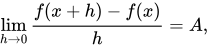
The Fréchet derivative defines the derivative for general normed vector spaces ${\displaystyle V,W}$. Briefly, a function ${\displaystyle f:U\to W}$, where ${\displaystyle U}$ is an open subset of ${\displaystyle V}$, is called Fréchet differentiable at ${\displaystyle x\in U}$ if there exists a bounded linear operator ${\displaystyle A:V\to W}$ such that $${\displaystyle \lim _{\|h\|\to 0}{\frac {\|f(x+h)-f(x)-Ah\|_{W}}{\|h\|_{V}}}=0.}$$

Functions are defined as being differentiable in some open neighbourhood of ${\displaystyle x}$, rather than at individual points, as not doing so tends to lead to many pathological counterexamples.

The Fréchet derivative is quite similar to the formula for the derivative found in elementary one-variable calculus, $${\displaystyle \lim _{h\to 0}{\frac {f(x+h)-f(x)}{h}}=A,}$$ and simply moves A to the left hand side. However, the Fréchet derivative A denotes the function ${\displaystyle t\mapsto f'(x)\cdot t}$.

In multivariable calculus, in the context of differential equations defined by a vector valued function Rⁿ to R^m, the Fréchet derivative A is a linear operator on R considered as a vector space over itself, and corresponds to the best linear approximation of a function. If such an operator exists, then it is unique, and can be represented by an m by n matrix known as the Jacobian matrix J_x(ƒ) of the mapping ƒ at point x. Each entry of this matrix represents a partial derivative, specifying the rate of change of one range coordinate with respect to a change in a domain coordinate. Of course, the Jacobian matrix of the composition g_°f is a product of corresponding Jacobian matrices: J_x(g_°f) =J_ƒ(x)(g)J_x(ƒ). This is a higher-dimensional statement of the chain rule.

For real valued functions from Rⁿ to R (scalar fields), the Fréchet derivative corresponds to a vector field called the total derivative. This can be interpreted as the gradient but it is more natural to use the exterior derivative.

The convective derivative takes into account changes due to time dependence and motion through space along a vector field, and is a special case of the total derivative.

For vector-valued functions from R to Rⁿ (i.e., parametric curves), the Fréchet derivative corresponds to taking the derivative of each component separately. The resulting derivative can be mapped to a vector. This is useful, for example, if the vector-valued function is the position vector of a particle through time, then the derivative is the velocity vector of the particle through time.

In complex analysis, the central objects of study are holomorphic functions, which are complex-valued functions on the complex numbers where the Fréchet derivative exists.

In geometric calculus, the geometric derivative satisfies a weaker form of the Leibniz (product) rule. It specializes the Fréchet derivative to the objects of geometric algebra. Geometric calculus is a powerful formalism that has been shown to encompass the similar frameworks of differential forms and differential geometry.^[1]

On the exterior algebra of differential forms over a smooth manifold, the exterior derivative is the unique linear map which satisfies a graded version of the Leibniz law and squares to zero. It is a grade 1 derivation on the exterior algebra. In R³, the gradient, curl, and divergence are special cases of the exterior derivative. An intuitive interpretation of the gradient is that it points "up": in other words, it points in the direction of fastest increase of the function. It can be used to calculate directional derivatives of scalar functions or normal directions. Divergence gives a measure of how much "source" or "sink" near a point there is. It can be used to calculate flux by divergence theorem. Curl measures how much "rotation" a vector field has near a point.

The Lie derivative is the rate of change of a vector or tensor field along the flow of another vector field. On vector fields, it is an example of a Lie bracket (vector fields form the Lie algebra of the diffeomorphism group of the manifold). It is a grade 0 derivation on the algebra.

Together with the interior product (a degree -1 derivation on the exterior algebra defined by contraction with a vector field), the exterior derivative and the Lie derivative form a Lie superalgebra.

In differential topology, a vector field may be defined as a derivation on the ring of smooth functions on a manifold, and a tangent vector may be defined as a derivation at a point. This allows the abstraction of the notion of a directional derivative of a scalar function to general manifolds. For manifolds that are subsets of Rⁿ, this tangent vector will agree with the directional derivative.

The differential or pushforward of a map between manifolds is the induced map between tangent spaces of those manifolds. It abstracts the Jacobian matrix.

In differential geometry, the covariant derivative makes a choice for taking directional derivatives of vector fields along curves. This extends the directional derivative of scalar functions to sections of vector bundles or principal bundles. In Riemannian geometry, the existence of a metric chooses a unique preferred torsion-free covariant derivative, known as the Levi-Civita connection. See also gauge covariant derivative for a treatment oriented to physics.

The exterior covariant derivative extends the exterior derivative to vector valued forms.

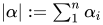
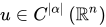
Given a function ${\displaystyle u:\mathbb {R} ^{n}\to \mathbb {R} }$ which is locally integrable, but not necessarily classically differentiable, a weak derivative may be defined by means of integration by parts. First define test functions, which are infinitely differentiable and compactly supported functions ${\displaystyle \varphi \in C_{c}^{\infty }\left(\mathbb {R} ^{n}\right)}$, and multi-indices, which are length ${\displaystyle n}$ lists of integers ${\displaystyle \alpha =(\alpha _{1},\dots ,\alpha _{n})}$ with ${\textstyle |\alpha |:=\sum _{1}^{n}\alpha _{i}}$. Applied to test functions, ${\textstyle D^{\alpha }\varphi :={\frac {\partial ^{|\alpha |}\varphi }{\partial x_{1}^{\alpha _{1}}\dotsm x_{n}^{\alpha _{n}}}}}$. Then the ${\textstyle \alpha ^{\text{th}}}$ weak derivative of ${\displaystyle u}$ exists if there is a function ${\displaystyle v:\mathbb {R} ^{n}\to \mathbb {R} }$ such that for all test functions ${\displaystyle \varphi }$, we have

${\displaystyle \int _{\mathbb {R} ^{n}}u\ D^{\alpha }\!\varphi \ dx=(-1)^{|\alpha |}\int _{\mathbb {R} ^{n}}v\ \varphi \ dx}$

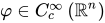
If such a function exists, then ${\displaystyle D^{\alpha }u:=v}$, which is unique almost everywhere. This definition coincides with the classical derivative for functions ${\displaystyle u\in C^{|\alpha |}\left(\mathbb {R} ^{n}\right)}$, and can be extended to a type of generalized functions called distributions, the dual space of test functions. Weak derivatives are particularly useful in the study of partial differential equations, and within parts of functional analysis.

In the real numbers one can iterate the differentiation process, that is, apply derivatives more than once, obtaining derivatives of second and higher order. Higher derivatives can also be defined for functions of several variables, studied in multivariable calculus. In this case, instead of repeatedly applying the derivative, one repeatedly applies partial derivatives with respect to different variables. For example, the second order partial derivatives of a scalar function of n variables can be organized into an n by n matrix, the Hessian matrix. One of the subtle points is that the higher derivatives are not intrinsically defined, and depend on the choice of the coordinates in a complicated fashion (in particular, the Hessian matrix of a function is not a tensor). Nevertheless, higher derivatives have important applications to analysis of local extrema of a function at its critical points. For an advanced application of this analysis to topology of manifolds, see Morse theory.

In addition to n th derivatives for any natural number n, there are various ways to define derivatives of fractional or negative orders, which are studied in fractional calculus. The −1 order derivative corresponds to the integral, whence the term differintegral.

In quaternionic analysis, derivatives can be defined in a similar way to real and complex functions. Since the quaternions ${\displaystyle \mathbb {H} }$ are not commutative, the limit of the difference quotient yields two different derivatives: A left derivative

${\displaystyle \lim _{h\to 0}\left[h^{-1}\left(f(a+h)-f(a)\right)\right]}$

and a right derivative

${\displaystyle \lim _{h\to 0}\left[\left(f(a+h)-f(a)\right)h^{-1}\right].}$

The existence of these limits are very restrictive conditions. For example, if ${\displaystyle f:\mathbb {H} \to \mathbb {H} }$ has left-derivatives at every point on an open connected set ${\displaystyle U\subset \mathbb {H} }$, then ${\displaystyle f(q)=a+qb}$ for ${\displaystyle a,b\in \mathbb {H} }$.

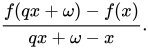
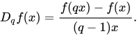
• The q-derivative of a function is defined by the formula $${\displaystyle D_{q}f(x)={\frac {f(qx)-f(x)}{(q-1)x}}.}$$ For x nonzero, if f is a differentiable function of x then in the limit as q → 1 we obtain the ordinary derivative, thus the q-derivative may be viewed as its q-deformation. A large body of results from ordinary differential calculus, such as binomial formula and Taylor expansion, have natural q-analogues that were discovered in the 19th century, but remained relatively obscure for a big part of the 20th century, outside of the theory of special functions. The progress of combinatorics and the discovery of quantum groups have changed the situation dramatically, and the popularity of q-analogues is on the rise.
• The difference operator of difference equations is another discrete analog of the standard derivative. $${\displaystyle \Delta f(x)=f(x+1)-f(x)}$$
• The q-derivative, the difference operator and the standard derivative can all be viewed as the same thing on different time scales. For example, taking ${\displaystyle \varepsilon =(q-1)x}$, we may have $${\displaystyle {\frac {f(qx)-f(x)}{(q-1)x}}={\frac {f(x+\varepsilon )-f(x)}{\varepsilon }}.}$$ The q-derivative is a special case of the Hahn difference,^[2] $${\displaystyle {\frac {f(qx+\omega )-f(x)}{qx+\omega -x}}.}$$The Hahn difference is not only a generalization of the q-derivative but also an extension of the forward difference.
• Also note that the q-derivative is nothing but a special case of the familiar derivative. Take ${\displaystyle z=qx}$. Then we have, $${\displaystyle \lim _{z\to x}{\frac {f(z)-f(x)}{z-x}}=\lim _{q\to 1}{\frac {f(qx)-f(x)}{qx-x}}=\lim _{q\to 1}{\frac {f(qx)-f(x)}{(q-1)x}}.}$$

In algebra, generalizations of the derivative can be obtained by imposing the Leibniz rule of differentiation in an algebraic structure, such as a ring or a Lie algebra.

A derivation is a linear map on a ring or algebra which satisfies the Leibniz law (the product rule). Higher derivatives and algebraic differential operators can also be defined. They are studied in a purely algebraic setting in differential Galois theory and the theory of D-modules, but also turn up in many other areas, where they often agree with less algebraic definitions of derivatives.

For example, the formal derivative of a polynomial over a commutative ring R is defined by

${\displaystyle \left(a_{d}x^{d}+a_{d-1}x^{d-1}+\cdots +a_{1}x+a_{0}\right)'=da_{d}x^{d-1}+(d-1)a_{d-1}x^{d-2}+\cdots +a_{1}.}$

The mapping ${\displaystyle f\mapsto f'}$ is then a derivation on the polynomial ring R[X]. This definition can be extended to rational functions as well.

The notion of derivation applies to noncommutative as well as commutative rings, and even to non-associative algebraic structures, such as Lie algebras.

In type theory, many abstract data types can be described as the algebra generated by a transformation that maps structures based on the type back into the type. For example, the type T of binary trees containing values of type A can be represented as the algebra generated by the transformation 1+A×T²→T. The "1" represents the construction of an empty tree, and the second term represents the construction of a tree from a value and two subtrees. The "+" indicates that a tree can be constructed either way.^[3][4]

The derivative of such a type is the type that describes the context of a particular substructure with respect to its next outer containing structure. Put another way, it is the type representing the "difference" between the two. In the tree example, the derivative is a type that describes the information needed, given a particular subtree, to construct its parent tree. This information is a tuple that contains a binary indicator of whether the child is on the left or right, the value at the parent, and the sibling subtree. This type can be represented as 2×A×T, which looks very much like the derivative of the transformation that generated the tree type.^[3][4]

This concept of a derivative of a type has practical applications, such as the zipper technique used in functional programming languages.^[3][4]

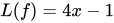
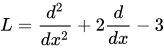
A differential operator combines several derivatives, possibly of different orders, in one algebraic expression. This is especially useful in considering ordinary linear differential equations with constant coefficients. For example, if f(x) is a twice differentiable function of one variable, the differential equation ${\displaystyle f''+2f'-3f=4x-1}$ may be rewritten in the form ${\displaystyle L(f)=4x-1}$, where $${\displaystyle L={\frac {d^{2}}{dx^{2}}}+2{\frac {d}{dx}}-3}$$ is a second order linear constant coefficient differential operator acting on functions of x. The key idea here is that we consider a particular linear combination of zeroth, first and second order derivatives "all at once". This allows us to think of the set of solutions of this differential equation as a "generalized antiderivative" of its right hand side 4x − 1, by analogy with ordinary integration, and formally write $${\displaystyle f(x)=L^{-1}(4x-1).}$$

Combining derivatives of different variables results in a notion of a partial differential operator. The linear operator which assigns to each function its derivative is an example of a differential operator on a function space. By means of the Fourier transform, pseudo-differential operators can be defined which allow for fractional calculus.

Some of these operators are so important that they have their own names:

• The Laplace operator or Laplacian on R³ is a second-order partial differential operator Δ given by the divergence of the gradient of a scalar function of three variables, or explicitly as $${\displaystyle \Delta ={\frac {\partial ^{2}}{\partial x^{2}}}+{\frac {\partial ^{2}}{\partial y^{2}}}+{\frac {\partial ^{2}}{\partial z^{2}}}.}$$ Analogous operators can be defined for functions of any number of variables.
• The d'Alembertian or wave operator is similar to the Laplacian, but acts on functions of four variables. Its definition uses the indefinite metric tensor of Minkowski space, instead of the Euclidean dot product of R³: $${\displaystyle \square ={\frac {\partial ^{2}}{\partial x^{2}}}+{\frac {\partial ^{2}}{\partial y^{2}}}+{\frac {\partial ^{2}}{\partial z^{2}}}-{\frac {1}{c^{2}}}{\frac {\partial ^{2}}{\partial t^{2}}}.}$$
• The Schwarzian derivative is a non-linear differential operator which describes how a complex function is approximated by a fractional-linear map, in much the same way that a normal derivative describes how a function is approximated by a linear map.
• The Wirtinger derivatives are a set of differential operators that permit the construction of a differential calculus for complex functions that is entirely analogous to the ordinary differential calculus for functions of real variables.

In functional analysis, the functional derivative defines the derivative with respect to a function of a functional on a space of functions. This is an extension of the directional derivative to an infinite dimensional vector space. An important case is the variational derivative in the calculus of variations.

The subderivative and subgradient are generalizations of the derivative to convex functions used in convex analysis.

In commutative algebra, Kähler differentials are universal derivations of a commutative ring or module. They can be used to define an analogue of exterior derivative from differential geometry that applies to arbitrary algebraic varieties, instead of just smooth manifolds.

In p-adic analysis, the usual definition of derivative is not quite strong enough, and one requires strict differentiability instead.

The Gateaux derivative extends the Fréchet derivative to locally convex topological vector spaces. Fréchet differentiability is a strictly stronger condition than Gateaux differentiability, even in finite dimensions. Between the two extremes is the quasi-derivative.

In measure theory, the Radon–Nikodym derivative generalizes the Jacobian, used for changing variables, to measures. It expresses one measure μ in terms of another measure ν (under certain conditions).

The H-derivative is a notion of derivative in the study of abstract Wiener spaces and the Malliavin calculus. It is used in the study of stochastic processes.

Laplacians and differential equations using the Laplacian can be defined on fractals. There is no completely satisfactory analog of the first-order derivative or gradient.^[5]

The Carlitz derivative is an operation similar to usual differentiation but with the usual context of real or complex numbers changed to local fields of positive characteristic in the form of formal Laurent series with coefficients in some finite field F_q (it is known that any local field of positive characteristic is isomorphic to a Laurent series field). Along with suitably defined analogs to the exponential function, logarithms and others the derivative can be used to develop notions of smoothness, analycity, integration, Taylor series as well as a theory of differential equations.^[6]

It may be possible to combine two or more of the above different notions of extension or abstraction of the original derivative. For example, in Finsler geometry, one studies spaces which look locally like Banach spaces. Thus one might want a derivative with some of the features of a functional derivative and the covariant derivative.

Multiplicative calculus replaces addition with multiplication, and hence rather than dealing with the limit of a ratio of differences, it deals with the limit of an exponentiation of ratios. This allows the development of the geometric derivative and bigeometric derivative. Moreover, just like the classical differential operator has a discrete analog, the difference operator, there are also discrete analogs of these multiplicative derivatives.

• Arithmetic derivative – Function defined on integers in number theory
• Automatic differentiation – Numerical calculations carrying along derivatives
• Brzozowski derivative – Function defined on formal languages in computer science
• Dini derivative – Class of generalisations of the derivative
• Fractal derivative – Generalization of derivative to fractals
• Hasse derivative – Mathematical concept
• Logarithmic derivative – Mathematical operation in calculus
• Logarithmic differentiation – Method of mathematical differentiation
• Non-classical analysis – Branch of mathematicsPages displaying short descriptions of redirect targets
• Numerical differentiation – Use of numerical analysis to estimate derivatives of functions
• Pincherle derivative – Type of derivative of a linear operator
• q-derivative – Q-analog of the ordinary derivative
• Semi-differentiability – Property of a mathematical function
• Symmetric derivative
• Topological derivative