At present, there is no single equation of state that accurately predicts the properties of all substances under all conditions. An example of an equation of state correlates densities of gases and liquids to temperatures and pressures, known as the ideal gas law, which is roughly accurate for weakly polar gases at low pressures and moderate temperatures. This equation becomes increasingly inaccurate at higher pressures and lower temperatures, and fails to predict condensation from a gas to a liquid.

The general form of an equation of state may be written as $${\displaystyle f(p,V,T)=0}$$

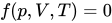
where ${\displaystyle p}$ is the pressure, ${\displaystyle V}$ the volume, and ${\displaystyle T}$ the temperature of the system. Yet also other variables may be used in that form. It is directly related to Gibbs phase rule, that is, the number of independent variables depends on the number of substances and phases in the system.

An equation used to model this relationship is called an equation of state. In most cases this model will comprise some empirical parameters that are usually adjusted to measurement data. Equations of state can also describe solids, including the transition of solids from one crystalline state to another. Equations of state are also used for the modeling of the state of matter in the interior of stars, including neutron stars, dense matter (quark–gluon plasmas) and radiation fields. A related concept is the perfect fluid equation of state used in cosmology.

Equations of state are applied in many fields such as process engineering and petroleum industry as well as pharmaceutical industry.

Any consistent set of units may be used, although SI units are preferred. Absolute temperature refers to the use of the Kelvin (K), with zero being absolute zero.

• ${\displaystyle n}$, number of moles of a substance
• ${\displaystyle V_{m}}$, ${\displaystyle {\frac {V}{n}}}$, molar volume, the volume of 1 mole of gas or liquid
• ${\displaystyle R}$, ideal gas constant ≈ 8.3144621 J/mol·K
• ${\displaystyle p_{c}}$, pressure at the critical point
• ${\displaystyle V_{c}}$, molar volume at the critical point
• ${\displaystyle T_{c}}$, absolute temperature at the critical point

Equations of state essentially began three centuries ago with the history of the ideal gas law:^[5]

$${\displaystyle pV=nRT}$$

Boyle's law was one of the earliest formulation of an equation of state. In 1662, the Irish physicist and chemist Robert Boyle performed a series of experiments employing a J-shaped glass tube, which was sealed on one end. Mercury was added to the tube, trapping a fixed quantity of air in the short, sealed end of the tube. Then the volume of gas was measured as additional mercury was added to the tube. The pressure of the gas could be determined by the difference between the mercury level in the short end of the tube and that in the long, open end. Through these experiments, Boyle noted that the gas volume varied inversely with the pressure. In mathematical form, this can be stated as:$${\displaystyle pV=\mathrm {constant} .}$$The above relationship has also been attributed to Edme Mariotte and is sometimes referred to as Mariotte's law. However, Mariotte's work was not published until 1676.

In 1787 the French physicist Jacques Charles found that oxygen, nitrogen, hydrogen, carbon dioxide, and air expand to roughly the same extent over the same 80-kelvin interval. This is known today as Charles's law. Later, in 1802, Joseph Louis Gay-Lussac published results of similar experiments, indicating a linear relationship between volume and temperature:$${\displaystyle {\frac {V_{1}}{T_{1}}}={\frac {V_{2}}{T_{2}}}.}$$Dalton's law (1801) of partial pressure states that the pressure of a mixture of gases is equal to the sum of the pressures of all of the constituent gases alone.

Mathematically, this can be represented for ${\displaystyle n}$ species as:$${\displaystyle p_{\text{total}}=p_{1}+p_{2}+\cdots +p_{n}=\sum _{i=1}^{n}p_{i}.}$$In 1834, Émile Clapeyron combined Boyle's law and Charles' law into the first statement of the ideal gas law. Initially, the law was formulated as pV_m = R(T_C + 267) (with temperature expressed in degrees Celsius), where R is the gas constant. However, later work revealed that the number should actually be closer to 273.2, and then the Celsius scale was defined with ${\displaystyle 0~^{\circ }\mathrm {C} =273.15~\mathrm {K} }$, giving:$${\displaystyle pV_{m}=R\left(T_{C}+273.15\ {}^{\circ }{\text{C}}\right).}$$In 1873, J. D. van der Waals introduced the first equation of state derived by the assumption of a finite volume occupied by the constituent molecules.^[6] His new formula revolutionized the study of equations of state, and was the starting point of cubic equations of state, which most famously continued via the Redlich–Kwong equation of state^[7] and the Soave modification of Redlich-Kwong.^[8]

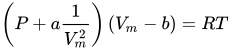
The van der Waals equation of state can be written as

$${\displaystyle \left(P+a{\frac {1}{V_{m}^{2}}}\right)(V_{m}-b)=RT}$$ where ${\displaystyle a}$ is a parameter describing the attractive energy between particles and ${\displaystyle b}$ is a parameter describing the volume of the particles.

The classical ideal gas law may be written $${\displaystyle pV=nRT.}$$

In the form shown above, the equation of state is thus $${\displaystyle f(p,V,T)=pV-nRT=0.}$$

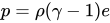
If the calorically perfect gas approximation is used, then the ideal gas law may also be expressed as follows $${\displaystyle p=\rho (\gamma -1)e}$$ where ${\displaystyle \rho }$ is the number density of the gas (number of atoms/molecules per unit volume), ${\displaystyle \gamma =C_{p}/C_{v}}$ is the (constant) adiabatic index (ratio of specific heats), ${\displaystyle e=C_{v}T}$ is the internal energy per unit mass (the "specific internal energy"), ${\displaystyle C_{v}}$ is the specific heat capacity at constant volume, and ${\displaystyle C_{p}}$ is the specific heat capacity at constant pressure.

Since for atomic and molecular gases, the classical ideal gas law is well suited in most cases, let us describe the equation of state for elementary particles with mass ${\displaystyle m}$ and spin ${\displaystyle s}$ that takes into account quantum effects. In the following, the upper sign will always correspond to Fermi–Dirac statistics and the lower sign to Bose–Einstein statistics. The equation of state of such gases with ${\displaystyle N}$ particles occupying a volume ${\displaystyle V}$ with temperature ${\displaystyle T}$ and pressure ${\displaystyle p}$ is given by^[9]

$${\displaystyle p={\frac {(2s+1){\sqrt {2m^{3}k_{\text{B}}^{5}T^{5}}}}{3\pi ^{2}\hbar ^{3}}}\int _{0}^{\infty }{\frac {z^{3/2}\,\mathrm {d} z}{e^{z-\mu /(k_{\text{B}}T)}\pm 1}}}$$ where ${\displaystyle k_{\text{B}}}$ is the Boltzmann constant and ${\displaystyle \mu (T,N/V)}$ the chemical potential is given by the following implicit function $${\displaystyle {\frac {N}{V}}={\frac {(2s+1)(mk_{\text{B}}T)^{3/2}}{{\sqrt {2}}\pi ^{2}\hbar ^{3}}}\int _{0}^{\infty }{\frac {z^{1/2}\,\mathrm {d} z}{e^{z-\mu /(k_{\text{B}}T)}\pm 1}}.}$$

In the limiting case where ${\displaystyle e^{\mu /(k_{\text{B}}T)}\ll 1}$, this equation of state will reduce to that of the classical ideal gas. It can be shown that the above equation of state in the limit ${\displaystyle e^{\mu /(k_{\text{B}}T)}\ll 1}$ reduces to

$${\displaystyle pV=Nk_{\text{B}}T\left[1\pm {\frac {\pi ^{3/2}}{2(2s+1)}}{\frac {N\hbar ^{3}}{V(mk_{\text{B}}T)^{3/2}}}+\cdots \right]}$$

With a fixed number density ${\displaystyle N/V}$, decreasing the temperature causes in Fermi gas, an increase in the value for pressure from its classical value implying an effective repulsion between particles (this is an apparent repulsion due to quantum exchange effects not because of actual interactions between particles since in ideal gas, interactional forces are neglected) and in Bose gas, a decrease in pressure from its classical value implying an effective attraction. The quantum nature of this equation is in it dependence on s and ħ.

Cubic equations of state are called such because they can be rewritten as a cubic function of ${\displaystyle V_{m}}$. Cubic equations of state originated from the van der Waals equation of state. Hence, all cubic equations of state can be considered 'modified van der Waals equation of state'. There is a very large number of such cubic equations of state. For process engineering, cubic equations of state are today still highly relevant, e.g. the Peng Robinson equation of state or the Soave Redlich Kwong equation of state.

$${\displaystyle {\frac {pV_{m}}{RT}}=A+{\frac {B}{V_{m}}}+{\frac {C}{V_{m}^{2}}}+{\frac {D}{V_{m}^{3}}}+\cdots }$$

Although usually not the most convenient equation of state, the virial equation is important because it can be derived directly from statistical mechanics. This equation is also called the Kamerlingh Onnes equation. If appropriate assumptions are made about the mathematical form of intermolecular forces, theoretical expressions can be developed for each of the coefficients. A is the first virial coefficient, which has a constant value of 1 and makes the statement that when volume is large, all fluids behave like ideal gases. The second virial coefficient B corresponds to interactions between pairs of molecules, C to triplets, and so on. Accuracy can be increased indefinitely by considering higher order terms. The coefficients B, C, D, etc. are functions of temperature only.

$${\displaystyle {\begin{aligned}p=\rho RT&+\left(B_{0}RT-A_{0}-{\frac {C_{0}}{T^{2}}}+{\frac {D_{0}}{T^{3}}}-{\frac {E_{0}}{T^{4}}}\right)\rho ^{2}+\left(bRT-a-{\frac {d}{T}}\right)\rho ^{3}\\[2pt]&+\alpha \left(a+{\frac {d}{T}}\right)\rho ^{6}+{\frac {c\rho ^{3}}{T^{2}}}\left(1+\gamma \rho ^{2}\right)\exp \left(-\gamma \rho ^{2}\right)\end{aligned}}}$$

where

• ${\displaystyle p}$ is pressure
• ${\displaystyle \rho }$ is molar density

Values of the various parameters can be found in reference materials.^[10] The BWR equation of state has also frequently been used for the modelling of the Lennard-Jones fluid.^[11][12] There are several extensions and modifications of the classical BWR equation of state available.

The Benedict–Webb–Rubin–Starling^[13] equation of state is a modified BWR equation of state and can be written as $${\displaystyle {\begin{aligned}p=\rho RT&+\left(B_{0}RT-A_{0}-{\frac {C_{0}}{T^{2}}}+{\frac {D_{0}}{T^{3}}}-{\frac {E_{0}}{T^{4}}}\right)\rho ^{2}\\[2pt]&+\left(bRT-a-{\frac {d}{T}}+{\frac {c}{T^{2}}}\right)\rho ^{3}+\alpha \left(a+{\frac {d}{T}}\right)\rho ^{6}\end{aligned}}}$$

Note that in this virial equation, the fourth and fifth virial terms are zero. The second virial coefficient is monotonically decreasing as temperature is lowered. The third virial coefficient is monotonically increasing as temperature is lowered.

The Lee–Kesler equation of state is based on the corresponding states principle, and is a modification of the BWR equation of state.^[14]

$${\displaystyle p={\frac {RT}{V}}\left(1+{\frac {B}{V_{r}}}+{\frac {C}{V_{r}^{2}}}+{\frac {D}{V_{r}^{5}}}+{\frac {c_{4}}{T_{r}^{3}V_{r}^{2}}}\left(\beta +{\frac {\gamma }{V_{r}^{2}}}\right)\exp \left(-{\frac {\gamma }{V_{r}^{2}}}\right)\right)}$$

There is a large number of physically based equations of state available today.^{[15][16][17][18][19][20][21][22]} Most of those are formulated in the Helmholtz free energy as a function of temperature, density (and for mixtures additionally the composition). The Helmholtz energy is formulated as a sum of multiple terms modelling different types of molecular interaction or molecular structures, e.g. the formation of chains or dipolar interactions. Hence, physically based equations of state model the effect of molecular size, attraction and shape as well as hydrogen bonding and polar interactions of fluids. In general, physically based equations of state give more accurate results than traditional cubic equations of state, especially for systems containing liquids or solids. Most physically based equations of state are built on monomer term describing the Lennard-Jones fluid or the Mie fluid.

Perturbation theory is frequently used for modelling dispersive interactions in an equation of state. There is a large number of perturbation theory based equations of state available today,^[23][24] e.g. for the classical Lennard-Jones fluid.^[11][25] The two most important theories used for these types of equations of state are the Barker-Henderson perturbation theory^[26] and the Weeks–Chandler–Andersen perturbation theory.^[27]

An important contribution for physically based equations of state is the statistical associating fluid theory (SAFT) that contributes the Helmholtz energy that describes the association (a.k.a. hydrogen bonding) in fluids, which can also be applied for modelling chain formation (in the limit of infinite association strength). The SAFT equation of state was developed using statistical mechanical methods (in particular the perturbation theory of Wertheim^[28]) to describe the interactions between molecules in a system.^[20][29][30] The idea of a SAFT equation of state was first proposed by Chapman et al. in 1988 and 1989.^[20][29][30] Many different versions of the SAFT models have been proposed, but all use the same chain and association terms derived by Chapman et al.^[29][31][32]

Multiparameter equations of state are empirical equations of state that can be used to represent pure fluids with high accuracy. Multiparameter equations of state are empirical correlations of experimental data and are usually formulated in the Helmholtz free energy. The functional form of these models is in most parts not physically motivated. They can be usually applied in both liquid and gaseous states. Empirical multiparameter equations of state represent the Helmholtz energy of the fluid as the sum of ideal gas and residual terms. Both terms are explicit in temperature and density: $${\displaystyle {\frac {a(T,\rho )}{RT}}={\frac {a^{\mathrm {ideal\,gas} }(\tau ,\delta )+a^{\textrm {residual}}(\tau ,\delta )}{RT}}}$$ with $${\displaystyle \tau ={\frac {T_{r}}{T}},\delta ={\frac {\rho }{\rho _{r}}}}$$

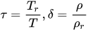
The reduced density ${\displaystyle \rho _{r}}$ and reduced temperature ${\displaystyle T_{r}}$ are in most cases the critical values for the pure fluid. Because integration of the multiparameter equations of state is not required and thermodynamic properties can be determined using classical thermodynamic relations, there are few restrictions as to the functional form of the ideal or residual terms.^[33][34] Typical multiparameter equations of state use upwards of 50 fluid specific parameters, but are able to represent the fluid's properties with high accuracy. Multiparameter equations of state are available currently for about 50 of the most common industrial fluids including refrigerants. The IAPWS95 reference equation of state for water is also a multiparameter equations of state.^[35] Mixture models for multiparameter equations of state exist, as well. Yet, multiparameter equations of state applied to mixtures are known to exhibit artifacts at times.^[36][37]

One example of such an equation of state is the form proposed by Span and Wagner.^[33]

$${\displaystyle {\begin{aligned}a^{\mathrm {residual} }={}&\sum _{i=1}^{8}\sum _{j=-8}^{12}n_{i,j}\delta ^{i}\tau ^{j/8}+\sum _{i=1}^{5}\sum _{j=-8}^{24}n_{i,j}\delta ^{i}\tau ^{j/8}\exp \left(-\delta \right)\\&+\sum _{i=1}^{5}\sum _{j=16}^{56}n_{i,j}\delta ^{i}\tau ^{j/8}\exp \left(-\delta ^{2}\right)+\sum _{i=2}^{4}\sum _{j=24}^{38}n_{i,j}\delta ^{i}\tau ^{j/2}\exp \left(-\delta ^{3}\right)\end{aligned}}}$$

This is a somewhat simpler form that is intended to be used more in technical applications.^[33] Equations of state that require a higher accuracy use a more complicated form with more terms.^[35][34]

When considering water under very high pressures, in situations such as underwater nuclear explosions, sonic shock lithotripsy, and sonoluminescence, the stiffened equation of state^[38] is often used:

$${\displaystyle p=\rho (\gamma -1)e-\gamma p^{0}\,}$$

where ${\displaystyle e}$ is the internal energy per unit mass, ${\displaystyle \gamma }$ is an empirically determined constant typically taken to be about 6.1, and ${\displaystyle p^{0}}$ is another constant, representing the molecular attraction between water molecules. The magnitude of the correction is about 2 gigapascals (20,000 atmospheres).

The equation is stated in this form because the speed of sound in water is given by ${\displaystyle c^{2}=\gamma \left(p+p^{0}\right)/\rho }$.

Thus water behaves as though it is an ideal gas that is already under about 20,000 atmospheres (2 GPa) pressure, and explains why water is commonly assumed to be incompressible: when the external pressure changes from 1 atmosphere to 2 atmospheres (100 kPa to 200 kPa), the water behaves as an ideal gas would when changing from 20,001 to 20,002 atmospheres (2000.1 MPa to 2000.2 MPa).

This equation mispredicts the specific heat capacity of water but few simple alternatives are available for severely nonisentropic processes such as strong shocks.

An equation of state of Morse oscillator has been derived,^[39] and it has the following form:

$${\displaystyle p=\Gamma _{1}\nu +\Gamma _{2}\nu ^{2}}$$

Where ${\displaystyle \Gamma _{1}}$ is the first order virial parameter and it depends on the temperature, ${\displaystyle \Gamma _{2}}$ is the second order virial parameter of Morse oscillator and it depends on the parameters of Morse oscillator in addition to the absolute temperature. ${\displaystyle \nu }$ is the fractional volume of the system.

An ultrarelativistic fluid has equation of state $${\displaystyle p=\rho _{m}c_{s}^{2}}$$ where ${\displaystyle p}$ is the pressure, ${\displaystyle \rho _{m}}$ is the mass density, and ${\displaystyle c_{s}}$ is the speed of sound.

The equation of state for an ideal Bose gas is

$${\displaystyle pV_{m}=RT~{\frac {\operatorname {Li} _{\alpha +1}(z)}{\zeta (\alpha )}}\left({\frac {T}{T_{c}}}\right)^{\alpha }}$$

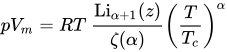
where α is an exponent specific to the system (e.g. in the absence of a potential field, α = 3/2), z is exp(μ/k_BT) where μ is the chemical potential, Li is the polylogarithm, ζ is the Riemann zeta function, and T_c is the critical temperature at which a Bose–Einstein condensate begins to form.

The equation of state from Jones–Wilkins–Lee is used to describe the detonation products of explosives. $${\displaystyle p=A\left(1-{\frac {\omega }{R_{1}V}}\right)\exp(-R_{1}V)+B\left(1-{\frac {\omega }{R_{2}V}}\right)\exp \left(-R_{2}V\right)+{\frac {\omega e_{0}}{V}}}$$

The ratio ${\displaystyle V=\rho _{e}/\rho }$ is defined by using ${\displaystyle \rho _{e}}$, which is the density of the explosive (solid part) and ${\displaystyle \rho }$, which is the density of the detonation products. The parameters ${\displaystyle A}$, ${\displaystyle B}$, ${\displaystyle R_{1}}$, ${\displaystyle R_{2}}$ and ${\displaystyle \omega }$ are given by several references.^[40] In addition, the initial density (solid part) ${\displaystyle \rho _{0}}$, speed of detonation ${\displaystyle V_{D}}$, Chapman–Jouguet pressure ${\displaystyle P_{CJ}}$ and the chemical energy per unit volume of the explosive ${\displaystyle e_{0}}$ are given in such references. These parameters are obtained by fitting the JWL-EOS to experimental results. Typical parameters for some explosives are listed in the table below.

Material	${\displaystyle \rho _{e}\,}$ (g/cm3)	${\displaystyle v_{D}\,}$ (m/s)	${\displaystyle p_{CJ}\,}$ (GPa)	${\displaystyle A\,}$ (GPa)	${\displaystyle B\,}$ (GPa)	${\displaystyle R_{1}}$	${\displaystyle R_{2}}$	${\displaystyle \omega }$	${\displaystyle e_{0}\,}$ (GPa)
TNT	1.630	6930	21.0	373.8	3.747	4.15	0.90	0.35	6.00
Composition B	1.717	7980	29.5	524.2	7.678	4.20	1.10	0.35	8.50
PBX 9501[41]	1.844		36.3	852.4	18.02	4.55	1.3	0.38	10.2

• Tait equation for water and other liquids. Several equations are referred to as the Tait equation.
• Murnaghan equation of state
• Birch–Murnaghan equation of state
• Stacey–Brennan–Irvine equation of state^[42]
• Modified Rydberg equation of state^[43][44][45]
• Adapted polynomial equation of state^[46]
• Johnson–Holmquist equation of state
• Mie–Grüneisen equation of state^[47][48]
• Anton-Schmidt equation of state
• State-transition equation

• Gas laws
• Departure function
• Table of thermodynamic equations
• Real gas
• Cluster expansion
• Polytrope