")
Community hub
Recent from talks
Contribute something
Nothing was collected or created yet.
Field (physics)
View on Wikipedia

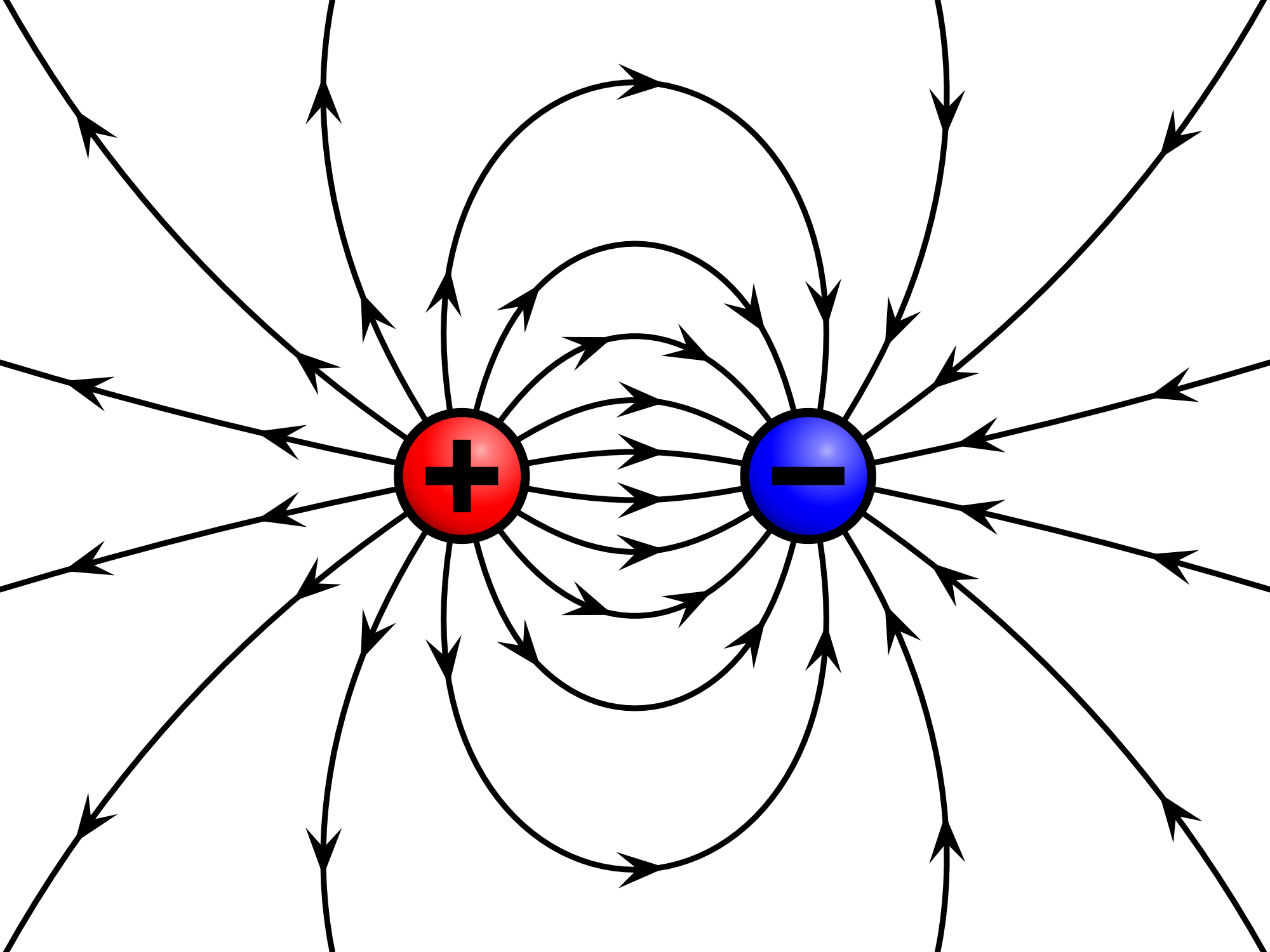
In science, a field is a physical quantity, represented by a scalar, vector, or tensor, that has a value for each point in space and time.[1][2][3] An example of a scalar field is a weather map, with the surface temperature described by assigning a number to each point on the map. A surface wind map,[4] assigning an arrow to each point on a map that describes the wind speed and direction at that point, is an example of a vector field, i.e. a 1-dimensional (rank-1) tensor field. Field theories, mathematical descriptions of how field values change in space and time, are ubiquitous in physics. For instance, the electric field is another rank-1 tensor field, while electrodynamics can be formulated in terms of two interacting vector fields at each point in spacetime, or as a single-rank 2-tensor field.[5][6][7]
In the modern framework of the quantum field theory, even without referring to a test particle, a field occupies space, contains energy, and its presence precludes a classical "true vacuum".[8] This has led physicists to consider electromagnetic fields to be a physical entity, making the field concept a supporting paradigm of the edifice of modern physics. Richard Feynman said, "The fact that the electromagnetic field can possess momentum and energy makes it very real, and [...] a particle makes a field, and a field acts on another particle, and the field has such familiar properties as energy content and momentum, just as particles can have."[9] In practice, the strength of most fields diminishes with distance, eventually becoming undetectable. For instance the strength of many relevant classical fields, such as the gravitational field in Newton's theory of gravity or the electrostatic field in classical electromagnetism, is inversely proportional to the square of the distance from the source (i.e. they follow Gauss's law).
A field can be classified as a scalar field, a vector field, a spinor field or a tensor field according to whether the represented physical quantity is a scalar, a vector, a spinor, or a tensor, respectively. A field has a consistent tensorial character wherever it is defined: i.e. a field cannot be a scalar field somewhere and a vector field somewhere else. For example, the Newtonian gravitational field is a vector field: specifying its value at a point in spacetime requires three numbers, the components of the gravitational field vector at that point. Moreover, within each category (scalar, vector, tensor), a field can be either a classical field or a quantum field, depending on whether it is characterized by numbers or quantum operators respectively. In this theory an equivalent representation of field is a field particle, for instance a boson.[10]
History
[edit]To Isaac Newton, his law of universal gravitation simply expressed the gravitational force that acted between any pair of massive objects. When looking at the motion of many bodies all interacting with each other, such as the planets in the Solar System, dealing with the force between each pair of bodies separately rapidly becomes computationally inconvenient. In the eighteenth century, a new quantity was devised to simplify the bookkeeping of all these gravitational forces. This quantity, the gravitational field, gave at each point in space the total gravitational acceleration which would be felt by a small object at that point. This did not change the physics in any way: it did not matter if all the gravitational forces on an object were calculated individually and then added together, or if all the contributions were first added together as a gravitational field and then applied to an object.[11] His idea in Opticks that optical reflection and refraction arise from interactions across the entire surface is arguably the beginning of the field theory of electric force.[12]
The development of the independent concept of a field truly began in the nineteenth century with the development of the theory of electromagnetism. In the early stages, André-Marie Ampère and Charles-Augustin de Coulomb could manage with Newton-style laws that expressed the forces between pairs of electric charges or electric currents. However, it became much more natural to take the field approach and express these laws in terms of electric and magnetic fields; in 1845 Michael Faraday became the first to coin the term "magnetic field".[13] And Lord Kelvin provided a formal definition for a field in 1851.[14]
The independent nature of the field became more apparent with James Clerk Maxwell's discovery that waves in these fields, called electromagnetic waves, propagated at a finite speed. Consequently, the forces on charges and currents no longer just depended on the positions and velocities of other charges and currents at the same time, but also on their positions and velocities in the past.[11]
Maxwell, at first, did not adopt the modern concept of a field as a fundamental quantity that could independently exist. Instead, he supposed that the electromagnetic field expressed the deformation of some underlying medium—the luminiferous aether—much like the tension in a rubber membrane. If that were the case, the observed velocity of the electromagnetic waves should depend upon the velocity of the observer with respect to the aether. Despite much effort, no experimental evidence of such an effect was ever found; the situation was resolved by the introduction of the special theory of relativity by Albert Einstein in 1905. This theory changed the way the viewpoints of moving observers were related to each other. They became related to each other in such a way that velocity of electromagnetic waves in Maxwell's theory would be the same for all observers. By doing away with the need for a background medium, this development opened the way for physicists to start thinking about fields as truly independent entities.[11]
In the late 1920s, the new rules of quantum mechanics were first applied to the electromagnetic field. In 1927, Paul Dirac used quantum fields to successfully explain how the decay of an atom to a lower quantum state led to the spontaneous emission of a photon, the quantum of the electromagnetic field. This was soon followed by the realization (following the work of Pascual Jordan, Eugene Wigner, Werner Heisenberg, and Wolfgang Pauli) that all particles, including electrons and protons, could be understood as the quanta of some quantum field, elevating fields to the status of the most fundamental objects in nature.[11] That said, John Wheeler and Richard Feynman seriously considered Newton's pre-field concept of action at a distance (although they set it aside because of the ongoing utility of the field concept for research in general relativity and quantum electrodynamics).
Classical fields
[edit]There are several examples of classical fields. Classical field theories remain useful wherever quantum properties do not arise, and can be active areas of research. Elasticity of materials, fluid dynamics and Maxwell's equations are cases in point.
Some of the simplest physical fields are vector force fields. Historically, the first time that fields were taken seriously was with Faraday's lines of force when describing the electric field. The gravitational field was then similarly described.
Newtonian gravitation
[edit].svg)
A classical field theory describing gravity is Newtonian gravitation, which describes the gravitational force as a mutual interaction between two masses.
Any body with mass M is associated with a gravitational field g which describes its influence on other bodies with mass. The gravitational field of M at a point r in space corresponds to the ratio between force F that M exerts on a small or negligible test mass m located at r and the test mass itself:[15]

Stipulating that m is much smaller than M ensures that the presence of m has a negligible influence on the behavior of M.
According to Newton's law of universal gravitation, F(r) is given by[15]

where is a unit vector lying along the line joining M and m and pointing from M to m. Therefore, the gravitational field of M is[15]


The experimental observation that inertial mass and gravitational mass are equal to an unprecedented level of accuracy leads to the identity that gravitational field strength is identical to the acceleration experienced by a particle. This is the starting point of the equivalence principle, which leads to general relativity.
Because the gravitational force F is conservative, the gravitational field g can be rewritten in terms of the gradient of a scalar function, the gravitational potential Φ(r):

Electromagnetism
[edit]Michael Faraday first realized the importance of a field as a physical quantity, during his investigations into magnetism. He realized that electric and magnetic fields are not only fields of force which dictate the motion of particles, but also have an independent physical reality because they carry energy.
These ideas eventually led to the creation, by James Clerk Maxwell, of the first unified field theory in physics with the introduction of equations for the electromagnetic field. The modern versions of these equations are called Maxwell's equations.
Electrostatics
[edit]A charged test particle with charge q experiences a force F based solely on its charge. We can similarly describe the electric field E so that F = qE. Using this and Coulomb's law tells us that the electric field due to a single charged particle is

The electric field is conservative, and hence can be described by a scalar potential, V(r):

Magnetostatics
[edit]A steady current I flowing along a path ℓ will create a field B, that exerts a force on nearby moving charged particles that is quantitatively different from the electric field force described above. The force exerted by I on a nearby charge q with velocity v is

where B(r) is the magnetic field, which is determined from I by the Biot–Savart law:

The magnetic field is not conservative in general, and hence cannot usually be written in terms of a scalar potential. However, it can be written in terms of a vector potential, A(r):


Electrodynamics
[edit]In general, in the presence of both a charge density ρ(r, t) and current density J(r, t), there will be both an electric and a magnetic field, and both will vary in time. They are determined by Maxwell's equations, a set of differential equations which directly relate E and B to ρ and J.[18]
Alternatively, one can describe the system in terms of its scalar and vector potentials V and A. A set of integral equations known as retarded potentials allow one to calculate V and A from ρ and J,[note 1] and from there the electric and magnetic fields are determined via the relations[19]


At the end of the 19th century, the electromagnetic field was understood as a collection of two vector fields in space. Nowadays, one recognizes this as a single antisymmetric 2nd-rank tensor field in spacetime.

Gravitation in general relativity
[edit].svg)
Einstein's theory of gravity, called general relativity, is another example of a field theory. Here the principal field is the metric tensor, a symmetric 2nd-rank tensor field in spacetime. This replaces Newton's law of universal gravitation.
Waves as fields
[edit]Waves can be constructed as physical fields, due to their finite propagation speed and causal nature when a simplified physical model of an isolated closed system is set [clarification needed]. They are also subject to the inverse-square law.
For electromagnetic waves, there are optical fields, and terms such as near- and far-field limits for diffraction. In practice though, the field theories of optics are superseded by the electromagnetic field theory of Maxwell.
Gravity waves are waves in the surface of water, defined by a height field.
Fluid dynamics
[edit]Fluid dynamics has fields of pressure, density, and flow rate that are connected by conservation laws for energy and momentum. The mass continuity equation is a continuity equation, representing the conservation of mass and the Navier–Stokes equations represent the conservation of momentum in the fluid, found from Newton's laws applied to the fluid, if the density ρ, pressure p, deviatoric stress tensor τ of the fluid, as well as external body forces b, are all given. The flow velocity u is the vector field to solve for.


Elasticity
[edit]Linear elasticity is defined in terms of constitutive equations between tensor fields,

where are the components of the 3 × 3 Cauchy stress tensor, the components of the 3 × 3 infinitesimal strain and is the elasticity tensor, a fourth-rank tensor with 81 components (usually 21 independent components).


Thermodynamics and transport equations
[edit]Assuming that the temperature T is an intensive quantity, i.e., a single-valued, differentiable function of three-dimensional space (a scalar field), i.e., that , then the temperature gradient is a vector field defined as . In thermal conduction, the temperature field appears in Fourier's law,


where q is the heat flux field and k the thermal conductivity.
Temperature and pressure gradients are also important for meteorology.
Quantum fields
[edit]It is now believed that quantum mechanics should underlie all physical phenomena, so that a classical field theory should, at least in principle, permit a recasting in quantum mechanical terms; success yields the corresponding quantum field theory. For example, quantizing classical electrodynamics gives quantum electrodynamics. Quantum electrodynamics is arguably the most successful scientific theory; experimental data confirm its predictions to a higher precision (to more significant digits) than any other theory.[22] The two other fundamental quantum field theories are quantum chromodynamics and the electroweak theory.
.svg)
In quantum chromodynamics, the color field lines are coupled at short distances by gluons, which are polarized by the field and line up with it. This effect increases within a short distance (around 1 fm from the vicinity of the quarks) making the color force increase within a short distance, confining the quarks within hadrons. As the field lines are pulled together tightly by gluons, they do not "bow" outwards as much as an electric field between electric charges.[23]
These three quantum field theories can all be derived as special cases of the so-called Standard Model of particle physics. General relativity, the Einsteinian field theory of gravity, has yet to be successfully quantized. However an extension, thermal field theory, deals with quantum field theory at finite temperatures, something seldom considered in quantum field theory.
In BRST theory one deals with odd fields, e.g. Faddeev–Popov ghosts. There are different descriptions of odd classical fields both on graded manifolds and supermanifolds.
As above with classical fields, it is possible to approach their quantum counterparts from a purely mathematical view using similar techniques as before. The equations governing the quantum fields are in fact PDEs (specifically, relativistic wave equations (RWEs)). Thus one can speak of Yang–Mills, Dirac, Klein–Gordon and Schrödinger fields as being solutions to their respective equations. A possible problem is that these RWEs can deal with complicated mathematical objects with exotic algebraic properties (e.g. spinors are not tensors, so may need calculus for spinor fields), but these in theory can still be subjected to analytical methods given appropriate mathematical generalization.
Field theory
[edit]Field theory usually refers to a construction of the dynamics of a field, i.e. a specification of how a field changes with time or with respect to other independent physical variables on which the field depends. Usually this is done by writing a Lagrangian or a Hamiltonian of the field, and treating it as a classical or quantum mechanical system with an infinite number of degrees of freedom. The resulting field theories are referred to as classical or quantum field theories.
The dynamics of a classical field are usually specified by the Lagrangian density in terms of the field components; the dynamics can be obtained by using the action principle.
It is possible to construct simple fields without any prior knowledge of physics using only mathematics from multivariable calculus, potential theory and partial differential equations (PDEs). For example, scalar PDEs might consider quantities such as amplitude, density and pressure fields for the wave equation and fluid dynamics; temperature/concentration fields for the heat/diffusion equations. Outside of physics proper (e.g., radiometry and computer graphics), there are even light fields. All these previous examples are scalar fields. Similarly for vectors, there are vector PDEs for displacement, velocity and vorticity fields in (applied mathematical) fluid dynamics, but vector calculus may now be needed in addition, being calculus for vector fields (as are these three quantities, and those for vector PDEs in general). More generally problems in continuum mechanics may involve for example, directional elasticity (from which comes the term tensor, derived from the Latin word for stretch), complex fluid flows or anisotropic diffusion, which are framed as matrix-tensor PDEs, and then require matrices or tensor fields, hence matrix or tensor calculus. The scalars (and hence the vectors, matrices and tensors) can be real or complex as both are fields in the abstract-algebraic/ring-theoretic sense.
In a general setting, classical fields are described by sections of fiber bundles and their dynamics is formulated in the terms of jet manifolds (covariant classical field theory).[24]
In modern physics, the most often studied fields are those that model the four fundamental forces which one day may lead to the Unified Field Theory.
Symmetries of fields
[edit]A convenient way of classifying a field (classical or quantum) is by the symmetries it possesses. Physical symmetries are usually of two types:
Spacetime symmetries
[edit]Fields are often classified by their behaviour under transformations of spacetime. The terms used in this classification are:
- scalar fields (such as temperature) whose values are given by a single variable at each point of space. This value does not change under transformations of space.
- vector fields (such as the magnitude and direction of the force at each point in a magnetic field) which are specified by attaching a vector to each point of space. The components of this vector transform between themselves contravariantly under rotations in space. Similarly, a dual (or co-) vector field attaches a dual vector to each point of space, and the components of each dual vector transform covariantly.
- tensor fields, (such as the stress tensor of a crystal) specified by a tensor at each point of space. Under rotations in space, the components of the tensor transform in a more general way which depends on the number of covariant indices and contravariant indices.
- spinor fields (such as the Dirac spinor) arise in quantum field theory to describe particles with spin which transform like vectors except for one of their components; in other words, when one rotates a vector field 360 degrees around a specific axis, the vector field turns to itself; however, spinors would turn to their negatives in the same case.
Internal symmetries
[edit]Fields may have internal symmetries in addition to spacetime symmetries. In many situations, one needs fields which are a list of spacetime scalars: (φ1, φ2, ... φN). For example, in weather prediction these may be temperature, pressure, humidity, etc. In particle physics, the color symmetry of the interaction of quarks is an example of an internal symmetry, that of the strong interaction. Other examples are isospin, weak isospin, strangeness and any other flavour symmetry.
If there is a symmetry of the problem, not involving spacetime, under which these components transform into each other, then this set of symmetries is called an internal symmetry. One may also make a classification of the charges of the fields under internal symmetries.
Statistical field theory
[edit]Statistical field theory attempts to extend the field-theoretic paradigm toward many-body systems and statistical mechanics. As above, it can be approached by the usual infinite number of degrees of freedom argument.
Much like statistical mechanics has some overlap between quantum and classical mechanics, statistical field theory has links to both quantum and classical field theories, especially the former with which it shares many methods. One important example is mean field theory.
Continuous random fields
[edit]Classical fields as above, such as the electromagnetic field, are usually infinitely differentiable functions, but they are in any case almost always twice differentiable. In contrast, generalized functions are not continuous. When dealing carefully with classical fields at finite temperature, the mathematical methods of continuous random fields are used, because thermally fluctuating classical fields are nowhere differentiable. Random fields are indexed sets of random variables; a continuous random field is a random field that has a set of functions as its index set. In particular, it is often mathematically convenient to take a continuous random field to have a Schwartz space of functions as its index set, in which case the continuous random field is a tempered distribution.
We can think about a continuous random field, in a (very) rough way, as an ordinary function that is almost everywhere, but such that when we take a weighted average of all the infinities over any finite region, we get a finite result. The infinities are not well-defined; but the finite values can be associated with the functions used as the weight functions to get the finite values, and that can be well-defined. We can define a continuous random field well enough as a linear map from a space of functions into the real numbers.

See also
[edit]Notes
[edit]- ^ This is contingent on the correct choice of gauge. V and A are not completely determined by ρ and J; rather, they are only determined up to some scalar function f(r, t) known as the gauge. The retarded potential formalism requires one to choose the Lorenz gauge.
References
[edit]- ^ John Gribbin (1998). Q is for Quantum: Particle Physics from A to Z. London: Weidenfeld & Nicolson. p. 138. ISBN 0-297-81752-3.
- ^ Richard Feynman (1970). The Feynman Lectures on Physics Vol II. Addison Wesley Longman. ISBN 978-0-201-02115-8.
A 'field' is any physical quantity which takes on different values at different points in space.
- ^ Ernan McMullin (2002). "The Origins of the Field Concept in Physics" (PDF). Phys. Perspect. 4 (1): 13–39. Bibcode:2002PhP.....4...13M. doi:10.1007/s00016-002-8357-5. S2CID 27691986.
- ^ SE, Windyty. "Windy as forecasted". Windy.com/. Retrieved 2021-06-25.
- ^ Lecture 1 | Quantum Entanglements, Part 1 (Stanford), Leonard Susskind, Stanford, Video, 2006-09-25.
- ^ Richard P. Feynman (1970). The Feynman Lectures on Physics Vol I. Addison Wesley Longman.
- ^ Richard P. Feynman (1970). The Feynman Lectures on Physics Vol II. Addison Wesley Longman.
- ^ John Archibald Wheeler (1998). Geons, Black Holes, and Quantum Foam: A Life in Physics. London: Norton. p. 163. ISBN 9780393046427.
- ^ Richard P. Feynman (1970). The Feynman Lectures on Physics Vol I. Addison Wesley Longman.
- ^ Steven Weinberg (November 7, 2013). "Physics: What We Do and Don't Know". New York Review of Books. 60 (17).
- ^ a b c d Weinberg, Steven (1977). "The Search for Unity: Notes for a History of Quantum Field Theory". Daedalus. 106 (4): 17–35. JSTOR 20024506.
- ^ Rowlands, Peter (2017). Newton – Innovation And Controversy. World Scientific Publishing. p. 109. ISBN 9781786344045.
- ^ Gooding, David (1 January 1981). "Final Steps to the Field Theory: Faraday's Study of Magnetic Phenomena, 1845-1850". Historical Studies in the Physical Sciences. 11 (2): 231–275. doi:10.2307/27757480. JSTOR 27757480.
- ^ McMullin, Ernan (February 2002). "[No title found]". Physics in Perspective. 4 (1): 13–39. Bibcode:2002PhP.....4...13M. doi:10.1007/s00016-002-8357-5.
- ^ a b c Kleppner, Daniel; Kolenkow, Robert. An Introduction to Mechanics. p. 85.
- ^ a b c Parker, C.B. (1994). McGraw Hill Encyclopaedia of Physics (2nd ed.). Mc Graw Hill. ISBN 0-07-051400-3.
- ^ a b c M. Mansfield; C. O’Sullivan (2011). Understanding Physics (4th ed.). John Wiley & Sons. ISBN 978-0-47-0746370.
- ^ Griffiths, David. Introduction to Electrodynamics (3rd ed.). p. 326.
- ^ Wangsness, Roald. Electromagnetic Fields (2nd ed.). p. 469.
- ^ J.A. Wheeler; C. Misner; K.S. Thorne (1973). Gravitation. W.H. Freeman & Co. ISBN 0-7167-0344-0.
- ^ I. Ciufolini; J.A. Wheeler (1995). Gravitation and Inertia. Princeton Physics Series. ISBN 0-691-03323-4.
- ^ Peskin, Michael E.; Schroeder, Daniel V. (1995). An Introduction to Quantum Fields. Westview Press. p. 198. ISBN 0-201-50397-2.. Also see precision tests of QED.
- ^ R. Resnick; R. Eisberg (1985). Quantum Physics of Atoms, Molecules, Solids, Nuclei and Particles (2nd ed.). John Wiley & Sons. p. 684. ISBN 978-0-471-87373-0.
- ^ Giachetta, G., Mangiarotti, L., Sardanashvily, G. (2009) Advanced Classical Field Theory. Singapore: World Scientific, ISBN 978-981-283-895-7 (arXiv:0811.0331)
Further reading
[edit]- "Fields". Principles of Physical Science. Vol. 25 (15th ed.). 1994. p. 815 – via Encyclopædia Britannica (Macropaedia).
- Landau, Lev D. and Lifshitz, Evgeny M. (1971). Classical Theory of Fields (3rd ed.). London: Pergamon. ISBN 0-08-016019-0. Vol. 2 of the Course of Theoretical Physics.
- Jepsen, Kathryn (July 18, 2013). "Real talk: Everything is made of fields" (PDF). Symmetry Magazine. Archived from the original (PDF) on March 4, 2016. Retrieved June 9, 2015.
External links
[edit]| International | |
|---|---|
| National | |
| Other | |
Field (physics)
View on GrokipediaDefinition and basic concepts
Core definition
In physics, a field is defined as a physical quantity that assigns a value—such as a scalar, vector, or tensor—to every point in spacetime, thereby describing how that quantity varies continuously across space and time.[9] This mapping represents physical entities like potentials, force densities, or energy distributions at each location, providing a framework for understanding extended interactions in the universe.[1] For instance, a scalar field might specify a temperature or gravitational potential at each point, while a vector field could indicate direction and magnitude, as in fluid velocity or electric field strength.[10] Fields are more than mathematical conveniences; they are physical entities that carry energy and momentum independently of the particles they influence, enabling the propagation of interactions through spacetime.[9] In contrast to viewing fields solely as tools to compute forces between discrete objects, modern physics treats them as fundamental components of reality, with their own dynamics governed by equations that ensure conservation laws like energy-momentum via Noether's theorem.[1] This perspective underscores fields' role as mediators, where distortions or excitations in the field exert forces on matter without requiring direct contact between sources.[10] A classic example is the Newtonian gravitational field strength near a point mass , given by where is the gravitational constant, is the distance from the mass, and is the unit radial vector pointing outward; this vector field points inward and decreases with distance, mediating the attractive force on a test mass as .[11] Similarly, the electromagnetic field assigns electric and magnetic vectors at each point, influencing charged particles through Lorentz forces without the charges needing to touch.[9] By conceptualizing distant interactions as local responses to field values at each point, fields unify phenomena that earlier action-at-a-distance models—such as instantaneous Newtonian gravity—struggled to explain coherently, providing a continuous medium for force propagation and energy transfer across the cosmos.[1] This approach eliminates paradoxes of infinite speed or direct influence over vast separations, instead allowing interactions to spread at finite speeds determined by the field's dynamics.[9]Mathematical representation
In physics, a field is formally represented as a smooth map , where is the spacetime manifold (typically a four-dimensional pseudo-Riemannian manifold) and is a vector space or more general fiber specifying the field's value type at each point . More abstractly, fields are sections of a fiber bundle over the spacetime base , where locally the section is parameterized as with coordinates on and fiber coordinates on . This framework ensures coordinate independence, as the field's tensorial nature dictates how it transforms under diffeomorphisms of .[12] Fields are classified by their transformation properties under the Lorentz group , which preserves the Minkowski metric in flat spacetime (and more generally under the structure group of the bundle). Scalar fields are invariant, transforming as . Vector fields (rank-1 contravariant) transform as , where is a Lorentz transformation matrix. Tensor fields of rank , such as the electromagnetic field strength , transform via the tensor product rule with contravariant and covariant indices. Spinor fields, like Dirac spinors , transform under the double-cover spin representation , enabling half-integer spin descriptions essential for fermions.[12][13] The dynamics of fields are encoded in partial differential equations (PDEs) derived from variational principles. For a real scalar field, a prototypical equation is the Klein-Gordon equation, where is the d'Alembertian operator in Minkowski metric , and is the field's mass parameter; this PDE describes a relativistic massive scalar particle. More generally, field equations arise from extremizing the action , where is the Lagrangian density, a scalar function depending on the field and its first derivatives. The Euler-Lagrange equations for a scalar field yield recovering PDEs like the Klein-Gordon for . For higher-rank fields, the formalism extends covariantly using jet bundles to incorporate derivatives.[12] To determine unique solutions to these hyperbolic PDEs, boundary conditions and initial value problems are imposed, ensuring well-posed evolution. Typically, initial data consist of the field configuration and its time derivative on a spacelike Cauchy hypersurface , satisfying constraints like vanishing Noether charges for local symmetries , where generates the symmetry. This setup allows time evolution via the field's propagation, respecting causality and energy conservation in the manifold's causal structure.[12]Historical development
Early concepts (pre-19th century)
The earliest precursors to the modern concept of a physical field emerged in ancient philosophy as intuitive notions of invisible, pervasive media that mediated natural motions in the cosmos. In the 4th century BCE, Aristotle proposed the ether as a fifth element, distinct from the terrestrial elements of earth, water, air, and fire, describing it as an eternal, divine substance that uniformly fills the celestial realm and imparts the natural circular motion to heavenly bodies.[14] This ether functioned as a continuous, unchanging medium, enabling the perpetual, frictionless revolutions of the stars and planets without alteration or decay, in contrast to the rectilinear, tendency-driven motions of sublunary objects.[14] Medieval scholastic thinkers built on Aristotelian foundations but began shifting toward more localized explanations of motion, hinting at forces tied to individual bodies rather than omnipresent media. In the 14th century, Jean Buridan refined the impetus theory in his commentaries on Aristotle's Physics, arguing that a thrown projectile sustains its path due to an "impetus"—an internal motive quality proportional to the object's weight and velocity—imparted by the thrower and diminishing only through external resistance like air.[15] Unlike Aristotle's reliance on surrounding media to propel objects, Buridan's impetus suggested a self-contained force residing within the body itself, diminishing over time without invoking a continuous enveloping influence, though it stopped short of a distributed field.[15] The 17th and 18th centuries saw intensified debates over action across distances, with Isaac Newton's gravitational theory in Philosophiæ Naturalis Principia Mathematica (1687) epitomizing instantaneous, non-mediated influence. Newton described gravity as a universal force attracting masses directly and immediately, proportional to their quantities and inversely to the square of their separation, without requiring contact or an intervening substance, thereby unifying the mechanics of falling apples and orbiting planets.[16] This action-at-a-distance framework, while empirically successful, provoked criticism for its apparent violation of mechanical principles, as it implied influences propagating through void space instantaneously.[16] In opposition, Gottfried Wilhelm Leibniz championed a relational view of space and the concept of vis viva (living force) as mv², positing it as the fundamental measure of a body's dynamic capacity to produce change, conserved in interactions and intrinsic to matter rather than externally imposed.[17] Leibniz rejected Newton's absolute space as an unnecessary container, arguing instead that space arises from the relational order among bodies, and he denounced gravitational action-at-a-distance as an occult, non-mechanical absurdity lacking sufficient reason or continuous mediation.[17] A complementary development came from Christiaan Huygens, who in 1678 outlined a wave theory of light in his unpublished Traité de la Lumière, conceiving light as longitudinal pressure waves propagating through a subtle, elastic luminiferous ether—an all-pervading medium analogous to air for sound waves.[18] This model implied field-like transmission, where local disturbances in the ether spread continuously outward at a finite speed, enabling phenomena like diffraction and refraction through the medium's uniform density and elasticity, rather than discrete particle emissions or instant effects.[18] These pre-19th-century ideas marked a philosophical progression from discrete, object-bound influences and static media toward continuous, distributed descriptions of propagation and interaction, paving the way for mathematical field theories.19th-century foundations
In the early 1820s, the connection between electricity and magnetism began to suggest the need for a mediating field concept. Danish physicist Hans Christian Ørsted discovered in 1820 that an electric current in a wire deflects a nearby compass needle, demonstrating that electricity produces magnetic effects, which he described in his seminal paper as a circumferential force around the current. This observation implied that magnetic influences propagate through space rather than acting instantaneously at a distance. Building on Ørsted's finding, French physicist André-Marie Ampère rapidly developed a mathematical theory of electrodynamics in 1820, proposing that electric currents interact via forces that could be modeled as arising from an intervening medium, prefiguring field mediation in his memoirs on current interactions.[19] By the 1830s, Michael Faraday's experimental investigations elevated the field idea from qualitative observation to a physical entity. Through extensive experiments on electromagnetic induction, Faraday introduced the concept of "lines of force" in his Experimental Researches in Electricity (starting 1831), visualizing magnetic and electric influences as tension lines pervading space, akin to physical realities in an ether rather than abstract actions.[20] These lines represented the direction and intensity of forces at every point, providing an intuitive framework for understanding how influences extend continuously through space without direct contact. Building directly on Faraday's lines of force, James Clerk Maxwell provided the mathematical foundation for electromagnetic fields in the 1860s. In his 1861 paper "On Physical Lines of Force," Maxwell modeled magnetic fields using rotating vortices in the luminiferous ether, with electric currents as their axes, and introduced displacement current to explain electromagnetic induction. His 1865 treatise "A Dynamical Theory of the Electromagnetic Field" unified electricity, magnetism, and light by deriving a set of equations—now known as Maxwell's equations—that describe how electric and magnetic fields interact and propagate as waves at the speed of light, establishing the electromagnetic field as a fundamental physical entity.[21] Mathematical formalization of fields emerged concurrently, drawing analogies to known physical systems. Siméon Denis Poisson had earlier derived in 1813 an equation for the gravitational potential Φ, ∇²Φ = 4πGρ, where ρ is mass density and G is the gravitational constant, which was later extended to describe fields as solutions to such partial differential equations governing potential distributions.[22] In the 1840s, William Thomson (later Lord Kelvin) advanced this by analogizing electric and magnetic fields to incompressible fluid flows, enabling the use of potential theory to quantify field behaviors in equilibrium, as detailed in his 1845 paper on heat and electricity analogies. Meanwhile, Hermann Grassmann's 1844 Die lineale Ausdehnungslehre introduced multilinear algebra for handling extended quantities, laying groundwork for non-scalar field descriptions beyond simple potentials. Bernhard Riemann further generalized this in his 1854 habilitation lecture, proposing metric tensors to describe geometric structures in n-dimensional spaces, which anticipated tensor fields for curved influences in physics.[23]20th-century unification
In 1905, Albert Einstein introduced special relativity, which reformulated classical field theories to ensure their invariance under Lorentz transformations, thereby eliminating the instantaneous action-at-a-distance inherent in Newtonian gravity and Maxwell's electrodynamics.[24] This framework unified space and time into Minkowski spacetime, where electromagnetic fields transform covariantly between inertial frames, providing a consistent description of fields propagating at the speed of light.[24] Einstein's approach resolved paradoxes in 19th-century electromagnetism by treating fields as fundamental entities distributed continuously in spacetime rather than as forces between distant particles.[24] Building on special relativity, Einstein developed general relativity in 1915, conceptualizing gravity as a curvature of spacetime induced by mass-energy, with the gravitational field encoded in the metric tensor.[25] The culmination of his efforts appeared in a series of papers that November, where he derived the Einstein field equations, relating the geometry of spacetime to the distribution of matter and energy: Here, is the Einstein tensor representing spacetime curvature, and is the stress-energy tensor. This formulation arose from Einstein's pursuit of general covariance, inspired by earlier work on equivalence principles and Riemannian geometry, marking a profound unification of gravity with the relativistic principles applied to other fields.[25] In the 1920s, Paul Dirac advanced the unification by developing a relativistic quantum theory of the electron, introducing the Dirac equation in 1928 as a first-order wave equation that combined quantum mechanics with special relativity.[26] This equation, , described the electron as a spin-1/2 field and naturally incorporated both positive and negative energy solutions, which Dirac interpreted as particles and antiparticles, predicting the existence of antimatter such as the positron.[26] Dirac's work bridged classical field theory and quantum mechanics, laying the groundwork for quantum field theory by treating particles as excitations of underlying fields.[26] The 1940s saw the maturation of quantum electrodynamics (QED) through the independent efforts of Sin-Itiro Tomonaga, Julian Schwinger, and Richard Feynman, who resolved infinities plaguing earlier quantum field calculations via renormalization techniques.[27] Tomonaga's 1946 covariant perturbation theory extended Dirac's framework to interacting fields, while Schwinger's 1948 canonical quantization and Feynman's 1949 path-integral diagrams provided practical methods to compute finite probabilities for processes like electron-photon scattering. Their unified approach, synthesized by Freeman Dyson, renormalized the electromagnetic field by redefining parameters like charge and mass to absorb divergences, yielding predictions accurate to many decimal places and establishing QED as the first successful relativistic quantum field theory.[27] By the 1970s, these developments converged in the Standard Model, which unified the electromagnetic and weak nuclear forces into a single electroweak interaction while incorporating the strong force via quantum chromodynamics.[28] Sheldon Glashow's 1961 SU(2) × U(1) gauge theory, refined by Steven Weinberg and Abdus Salam in 1967–1968 through spontaneous symmetry breaking via the Higgs mechanism, predicted massive W and Z bosons mediating weak interactions alongside the massless photon. The model's emergence was confirmed by the 1973 discovery of neutral currents and culminated in the 1983 detection of W and Z bosons at CERN, integrating quantum fields for quarks, leptons, and gauge bosons into a cohesive framework describing three of the four fundamental forces.[28]Classical field theories
Gravitational fields
In Newtonian physics, the gravitational field describes the gravitational influence of a mass distribution on a test particle, manifesting as an acceleration experienced by the particle. The gravitational field at a point is defined as the force per unit mass on a test mass placed there, and it can be derived from a scalar gravitational potential via . For a point mass at the origin, the potential is , where is the gravitational constant and , yielding .[29][30] The behavior of the gravitational field is governed by two fundamental equations analogous to those in electrostatics. The divergence of the field relates to the mass density through Gauss's law for gravity: , indicating that mass acts as a source for the field's divergence. Additionally, the field is irrotational, satisfying , which implies the existence of the potential and conservative nature of the force. Substituting into the divergence equation yields Poisson's equation: . These equations hold for any mass distribution, with the field at a point computed by integrating contributions from all masses.[31][32] The gravitational field represents the acceleration imparted to any test mass due to the surrounding mass distribution, independent of the test mass's value, underscoring the universality of free fall. For multiple sources, the total field follows the superposition principle: the net is the vector sum of fields from each source, a direct consequence of the linearity of Newton's law of universal gravitation, , extended to fields. This principle enables the calculation of complex systems by adding individual contributions, as seen in planetary systems where the Sun's field dominates but perturbations from other planets are superposed.[30]/02:_Review_of_Newtonian_Mechanics/2.14:_Newton's_Law_of_Gravitation) Gravitational fields carry energy and momentum, analogous to other classical fields. The energy density stored in the field is , where , reflecting the negative potential energy associated with gravitational attraction; the total field energy is obtained by integrating this density over all space. This formulation arises from expressing the interaction energy between masses in terms of the field, ensuring conservation in isolated systems. Momentum density in the field, though zero for static configurations, becomes relevant in dynamic cases but remains secondary in the Newtonian limit.[33] Despite its successes, Newtonian gravitational fields have key limitations. The theory assumes instantaneous propagation of gravitational influences across distances, violating causality in modern physics where interactions are finite-speed. It also fails in regimes of high velocities or strong fields; for instance, the predicted orbit of Mercury shows a perihelion advance of only about 532 arcseconds per century from planetary perturbations, falling short of the observed 575 arcseconds, with the 43-arcsecond discrepancy unresolved until later theories. These shortcomings highlight the approximation's validity only for weak fields and low speeds relative to light.[34][35] Applications of Newtonian gravitational fields abound in classical mechanics. In orbital mechanics, the field governs the motion of satellites and planets, leading to Kepler's laws as solutions to for central forces, enabling precise predictions of trajectories in solar system dynamics. Tidal forces, arising from the nonuniformity of the field across an extended body, cause deformations; for Earth-Moon-Sun interactions, the differential produces ocean bulges, with the Moon's tidal acceleration roughly twice the Sun's due to proximity despite lower mass. These effects are quantified by the tidal tensor, derived from second derivatives of , and underpin phenomena like tidal locking in binary systems./Book:University_Physics_I-Mechanics_Sound_Oscillations_and_Waves(OpenStax)/13:_Gravitation/13.07:_Tidal_Forces)Electromagnetic fields
The electromagnetic field unifies the electric field , which exerts forces on stationary charges, and the magnetic field , which affects moving charges and is generated by currents.[36] These fields are described in classical electromagnetism through the four-potential , where is the scalar potential and is the vector potential, from which and .[37] In covariant form, the electromagnetic field is captured by the antisymmetric tensor , whose components encode both and .[37] This formulation, rooted in 19th-century developments by James Clerk Maxwell, provides a compact representation of the unified field.[38] In static cases, where fields do not vary with time, the electric field obeys Coulomb's law, and , with the vacuum permittivity, describing divergence from charges and irrotational nature.[36] Similarly, magnetostatics follows and , where is the vacuum permeability and the current density, indicating no magnetic monopoles and circulation around currents.[36] These relations stem from empirical laws integrated into Maxwell's framework.[38] For dynamic situations, Maxwell's equations fully govern the fields: , , , and .[36] The added displacement current term enables wave propagation, predicting transverse electromagnetic waves traveling at speed m/s in vacuum, matching the speed of light.[38][39][40] Energy flow in these waves is given by the Poynting vector , where , representing the directional flux of electromagnetic energy.[41] Charges and currents experience the Lorentz force , combining electric and magnetic contributions, which drives particle motion in the field.[42] This force law, derived from experimental observations and Maxwell's theory, underscores the field's role in mediating interactions between charged particles.[42]Continuum mechanics fields
In continuum mechanics, fields describe the macroscopic behavior of deformable media such as fluids and solids, where properties like velocity, density, and stress vary continuously across space and time, emerging from the collective motion of constituent particles. These fields are classical and non-fundamental, governed by conservation laws and constitutive relations that model interactions at scales much larger than atomic distances. Unlike microscopic fields tied to fundamental forces, continuum fields approximate the medium as a smooth distribution, enabling the analysis of phenomena like flow and deformation without resolving individual molecules. In fluid dynamics, the velocity field represents the local velocity at position and time , satisfying the Navier-Stokes equations, which express Newton's second law for viscous fluids: where is density, is pressure, is dynamic viscosity, and denotes body forces. These equations were first derived by Claude-Louis Navier in his 1822 memoir on fluid motion, incorporating molecular interactions via a viscous stress term, and rigorously justified by George Gabriel Stokes in 1845 through considerations of internal friction.[43][44] Accompanying the velocity field are the scalar density field and pressure field , linked by the continuity equation, which enforces mass conservation: This equation, originating from Leonhard Euler's 1757 principles of fluid motion, ensures that local changes in density balance the divergence of mass flux, forming the foundation for incompressible and compressible flow analyses.[45] For solids, elastic fields capture deformation under applied loads, with the displacement field denoting the vector shift of material points from their reference positions. The infinitesimal strain tensor, a symmetric measure of local deformation, is given by as introduced by Augustin-Louis Cauchy in his 1822 work on continuum equilibrium, approximating small strains where rotations are negligible. The stress tensor , representing internal forces per unit area, relates to strain via Hooke's law for isotropic linear elasticity: where and are the Lamé constants, with as the shear modulus and accounting for volumetric changes; these parameters were formalized by Gabriel Lamé in 1833 to generalize uniaxial Hookean behavior to three dimensions. Equilibrium requires , balancing stresses with inertia and body forces. Wave fields in continua arise from linearized perturbations, such as acoustic waves propagating through fluids or solids, where small-amplitude disturbances in pressure or displacement satisfy wave equations derived from the full dynamical equations. In fluids, the speed of acoustic waves is , with as the bulk modulus measuring resistance to compression; this adiabatic relation was established by Pierre-Simon Laplace in 1816, correcting Isaac Newton's isothermal assumption to match experimental speeds in air. For solids, longitudinal waves travel at , highlighting how elastic moduli dictate propagation. These fields model sound transmission, with plane-wave solutions where .[46] Thermodynamic fields, such as the temperature field , govern heat transfer in continua via the heat equation with as thermal diffusivity; this diffusion equation was derived by Joseph Fourier in 1822, based on the assumption of heat flux proportional to temperature gradient (Fourier's law). Similarly, mass diffusion of a concentration field , as in solute transport, follows Fick's second law where is the diffusion coefficient, analogous to and formulated by Adolf Fick in 1855 by analogy to heat conduction, treating diffusive flux as . These parabolic equations predict smoothing over time, essential for modeling thermal and chemical equilibration in media.[47][48]Relativistic extensions
Fields in special relativity
In special relativity, physical fields are described within the framework of four-dimensional Minkowski spacetime, where coordinates are combined into a four-vector and fields must transform under the Lorentz group to preserve the invariance of the spacetime interval .[49] This transformation ensures that physical laws remain consistent across inertial frames moving at constant velocities relative to each other, with the Lorentz group acting on four-vectors such as the four-momentum , where is the energy and is the three-momentum.[50] Classical fields, like those in electromagnetism, serve as a starting point for this relativistic formulation, requiring adaptation to covariant tensor representations.[51] Scalar fields in special relativity are the simplest Lorentz-invariant objects, satisfying the Klein-Gordon equation , where is the d'Alembertian operator and is the scalar field with mass . This wave equation arises from combining the relativistic energy-momentum relation with the quantum correspondence and , but in the classical context, it describes free propagating scalar disturbances invariant under Lorentz transformations.[52] For interacting cases, sources can be added covariantly, maintaining the equation's second-order hyperbolic form. Vector fields, such as the electromagnetic field, are represented by the four-potential , where is the scalar potential and is the vector potential, transforming as a four-vector under Lorentz boosts.[53] The electromagnetic field strength tensor is then a Lorentz-invariant antisymmetric tensor, encapsulating the electric and magnetic fields in a unified way: and .[53] Maxwell's equations reformulate covariantly as and , ensuring gauge invariance and relativistic consistency.[51] In relativistic mechanics influenced by fields, the four-force generalizes the three-force, where is proper time and the four-momentum responds to field interactions while remaining orthogonal to the four-velocity such that .[54] For electromagnetic fields, this yields , linking field tensors directly to particle dynamics in a covariant manner.[55] Causality in relativistic field theories is enforced by the finite speed of light , with field propagators and influences confined to or within light cones in spacetime, defining domains of dependence where future events at a point are determined only by initial data in the past light cone.[56] This structure prevents superluminal signaling, as hyperbolic partial differential equations like those governing fields ensure solutions propagate at speeds , preserving the chronological order of causally connected events across frames.[57] Violations would contradict the Lorentz invariance fundamental to special relativity.Fields in general relativity
In general relativity, gravity is not described by a vector field as in Newtonian mechanics but by the curvature of spacetime itself, represented as a tensor field known as the metric tensor . This symmetric second-rank tensor defines the infinitesimal proper distance in a four-dimensional pseudo-Riemannian manifold, thereby encoding the geometry that governs the motion of matter and light. The metric tensor determines the spacetime structure, with its components varying across coordinates to reflect gravitational influences, distinguishing general relativity from the flat Minkowski spacetime of special relativity. The connection between the metric and the geometry is mediated by the Christoffel symbols of the second kind, , which quantify how coordinate bases change under parallel transport and define the Levi-Civita connection for torsion-free spaces. These symbols arise directly from the metric derivatives and are essential for computing curvature without introducing additional fields. The dynamics of the gravitational field are then governed by the Einstein field equations, , where is the Ricci curvature tensor, is the Ricci scalar, is the gravitational constant, is the speed of light, and is the stress-energy tensor representing matter and energy sources. These equations, finalized by Einstein in late 1915, dictate how the curvature (left side) responds to the distribution of mass-energy (right side), unifying geometry with physics.[58] Matter and light follow paths of extremal proper length in this curved geometry, known as geodesics, satisfying the equation derived from varying the line element such that for null geodesics (like light paths) or timelike for massive particles. In the weak-field limit, where gravitational potentials are small, the metric component (with the Newtonian gravitational potential) recovers the Newtonian description, confirming consistency with classical gravity for low velocities and weak fields. Exact solutions to the field equations reveal extreme manifestations of the gravitational field, such as black holes and singularities; for instance, the Schwarzschild metric for a spherically symmetric, non-rotating mass is given by where , describing the spacetime around a point mass and featuring an event horizon at . This solution, derived shortly after the field equations, illustrates how the tensor field can produce regions of inescapable curvature.Quantum field theories
Quantization of classical fields
In the quantization of classical fields, the classical description is transformed into a quantum mechanical framework by treating the fields as operators on a Hilbert space, thereby incorporating the principles of quantum mechanics such as uncertainty and superposition. This approach bridges classical field theories, like those for electromagnetism or scalar fields, with quantum field theory, enabling the description of particles as excitations of underlying fields. The foundational method, canonical quantization, involves promoting the field variables and their conjugate momenta to non-commuting operators, ensuring consistency with the Heisenberg uncertainty principle. Canonical quantization proceeds by identifying the Lagrangian density ℒ of the classical theory, defining the canonical momentum π = ∂ℒ/∂(∂₀φ) conjugate to the field φ, and then imposing operator commutation relations [φ̂(x), π̂(y)] = iℏ δ³(x - y) at equal times t = 0, while other commutators vanish. This procedure was introduced by Paul Dirac in his 1927 paper on the quantum theory of radiation, where he applied it to the electromagnetic field to resolve inconsistencies in early quantum electrodynamics. The resulting quantum theory satisfies the classical equations of motion in the Heisenberg picture, but introduces non-classical features like field fluctuations. Second quantization extends this formalism by interpreting particles as creation and annihilation operators acting on the field, allowing for variable particle number and relativistic invariance. In this picture, the field operator is expanded in terms of modes, and particles emerge as quanta of these modes, with bosonic creation and annihilation operators â†_p and â_p satisfying [â_p, â†_q] = δ³(p - q), while the number operator for a mode is N = ↠â, counting particle occupation. This concept was developed by Pascual Jordan in 1927, building on Dirac's work, to handle many-body systems and field interactions systematically. For fermions, anticommutation relations {â_p, â†_q} = δ³(p - q) replace the commutators, as formalized by Jordan and Eugene Wigner in 1928. A concrete example is the quantization of the Klein-Gordon field for a real scalar field obeying (□ + m²)φ = 0. The field operator is expressed in momentum space as where \omega_p = \sqrt{\mathbf{p}^2 c^2 + m^2 c^4}/\hbar is the angular frequency corresponding to the energy E_p = \hbar \omega_p, and the operators satisfy [â_p, â†_q] = (2\pi \hbar)^3 δ³(p - q). This expansion, derived via canonical quantization, was first outlined by Jordan and Wolfgang Pauli in their 1928 treatment of radiation fields, treating the scalar field as a simplified model for photons. The vacuum state |0⟩ is defined by â_p |0⟩ = 0 for all p, representing the ground state with no particles. An alternative formulation is the path integral approach, where the quantum theory is defined by summing over all possible field configurations weighted by the phase factor from the action. The partition function is Z = ∫ Dφ exp(i S[φ]/ℏ), with S[φ] = ∫ d⁴x ℒ the classical action, and correlation functions obtained as functional derivatives of Z. This method, introduced by Richard Feynman in 1948 for non-relativistic quantum mechanics and extended to fields, provides a perturbative framework via Feynman diagrams and avoids explicit operator ordering ambiguities. It generates the same S-matrix elements as canonical quantization for renormalizable theories. A key consequence of quantization is vacuum fluctuations, where the vacuum state exhibits non-zero energy due to zero-point contributions from all modes, leading to the infinite zero-point energy E_0 = (1/2) ∑ ω_p, regularized via renormalization. These fluctuations manifest physically, as in the Lamb shift or Casimir effect, and arise inherently from the commutation relations in the quantized field.[59]Standard Model fields
The Standard Model of particle physics describes the fundamental interactions via a set of quantum fields, encompassing gauge fields for force mediation, fermion fields for matter constituents, and the Higgs field for mass generation. These fields are organized under the gauge group SU(3)_C × SU(2)_L × U(1)_Y, where SU(3)_C governs the strong force, and SU(2)_L × U(1)_Y unifies the weak and electromagnetic forces.[60][61] Gauge fields include the gluons, which are eight massless vector bosons transforming under the adjoint representation of SU(3)_C and mediating the strong interaction between color-charged particles.[61] The electroweak sector features three massive vector bosons—W⁺, W⁻ (charged, with mass M_W ≈ 80.4 GeV), and Z (neutral, with mass M_Z ≈ 91.2 GeV)—arising from SU(2)_L × U(1)_Y, along with the massless photon mediating electromagnetism under U(1)_EM.[60] Fermion fields consist of quarks and leptons, all described as Dirac spinors with six flavors each, arranged in three generations. Quarks (up, down, charm, strange, top, bottom) carry color charge and transform under the fundamental representation of SU(3)_C, with left-handed components in SU(2)_L doublets (e.g., (u_L, d_L)) and right-handed as singlets.[61] Leptons (electron, muon, tau, and their neutrinos) lack color charge, with left-handed doublets (e.g., (ν_eL, e_L)) and right-handed singlets, enabling chiral interactions in the weak sector.[60] The Higgs field is a complex scalar SU(2)_L doublet Φ with hypercharge Y=1, featuring four real degrees of freedom.[62] Spontaneous symmetry breaking occurs when the neutral component acquires a vacuum expectation value ⟨Φ⟩ = (0, v/√2)^T, with v ≈ 246 GeV, breaking SU(2)_L × U(1)_Y to U(1)_EM and generating masses for W, Z, and fermions via m_f = y_f v / √2, where y_f is the Yukawa coupling; the remaining degree of freedom manifests as the Higgs boson with mass ≈ 125 GeV.[62][60] The Standard Model Lagrangian is ℒ_SM = ℒ_gauge + ℒ_fermion + ℒ_Higgs + ℒ_Yukawa, where the gauge part includes −(1/4) F^a_{μν} F^{a μν} for non-Abelian fields (summed over gluons and electroweak bosons) and the Abelian photon term.[61][60] Fermion terms involve covariant derivatives and Yukawa couplings −∑ y_f \bar{ψ}_L Φ ψ_R + h.c., while ℒ_Higgs = (D_μ Φ)^† (D^μ Φ) − V(Φ) with V(Φ) = −μ² Φ† Φ + λ (Φ† Φ)^2.[62] Key interactions include quantum chromodynamics (QCD) confinement, where the strong force binds quarks and gluons into color-singlet hadrons due to the non-Abelian nature of SU(3)_C, exhibiting asymptotic freedom at high energies.[61] Electroweak unification enables charged-current weak interactions via W bosons and neutral currents via Z, predicting the Z mass through precision electroweak measurements.[60]Advanced topics in field theory
Symmetries and field transformations
In field theory, symmetries play a fundamental role in determining the structure of physical laws and the conservation properties of systems. A key principle linking symmetries to conservation laws is Noether's theorem, which states that every continuous symmetry of the action functional leads to a corresponding conserved current. Specifically, for a symmetry transformation parameterized by an infinitesimal parameter , the theorem yields a conserved Noether current satisfying , where the conservation arises from the invariance of the action under the transformation.[63] For example, spacetime translations correspond to conservation of the energy-momentum tensor , with , reflecting the homogeneity of space and time.[63] Spacetime symmetries are embodied in the Poincaré group, which combines Lorentz transformations and translations, forming the foundational symmetry group of special relativity. Fields in relativistic theories transform under irreducible unitary representations of this group, ensuring the invariance of the action under Poincaré transformations. This invariance dictates the form of field equations, such as the Klein-Gordon or Dirac equations, where the Lagrangian density is constructed to be scalar under Lorentz boosts and rotations, while translations enforce translational invariance. The Poincaré group's structure guarantees that physical observables, like particle masses and spins, classify under its representations, with massive particles corresponding to the little group SO(3) and massless ones to ISO(2). Internal symmetries, distinct from spacetime ones, act on the internal degrees of freedom of fields without affecting coordinates. A prominent example is the global U(1) symmetry, under which a complex scalar field transforms as for constant , leading via Noether's theorem to conservation of charge, with the current .[64] Promoting this to a local gauge symmetry, where varies with position, requires the introduction of a gauge field to maintain invariance, achieved through the covariant derivative , where is the coupling constant. This local U(1) invariance underpins quantum electrodynamics, with the gauge field becoming the photon. More generally, non-Abelian internal symmetries, such as SU(2), extend this framework, as in the Yang-Mills theory, where the structure group dictates the self-interacting nature of gauge bosons.[64] When a continuous symmetry is spontaneously broken—meaning the vacuum state is not invariant under the symmetry transformation, while the Lagrangian remains so—Nambu-Goldstone bosons emerge as massless excitations. The Goldstone theorem asserts that for each broken generator of a continuous symmetry, there exists a massless scalar field, corresponding to the modes that restore the broken symmetry in the low-energy effective theory.[65] These bosons arise in systems like the Higgs mechanism in the electroweak theory, where the broken symmetry generates longitudinal components for massive gauge bosons, though the theorem's massless prediction holds in the absence of gauge coupling.[65] Modern extensions include conformal symmetries, which enlarge the Poincaré group by requiring scale invariance in addition to Lorentz and translational invariance, leading to conserved currents associated with dilatations and special conformal transformations; these are crucial in conformal field theories describing critical phenomena. Supersymmetry transformations further unify bosonic and fermionic fields, positing a symmetry between their statistics, with the super-Poincaré group extending spacetime symmetries to include fermionic generators, yielding conserved supercharges via Noether's theorem in supersymmetric field theories.Statistical and random fields
Statistical field theory employs path integrals to compute partition functions in systems with many degrees of freedom, where the partition function is expressed as , with denoting the Euclidean action and the integral over all field configurations . This formalism bridges classical statistical mechanics and quantum field theory by treating the path integral as an ensemble average over fluctuating fields, enabling the study of thermodynamic properties through effective actions obtained by integrating out high-momentum modes.[66] A prototypical example is the Ising model on a lattice, where spins represent a discrete field, and its continuum limit yields the theory, described by the action , capturing phase transitions in ferromagnets. Critical exponents governing the behavior near the transition, such as the specific heat exponent or correlation length exponent , are determined using the renormalization group (RG) approach, which rescales the theory to reveal fixed points and scaling laws; for the 3D Ising model, RG predictions yield . This continuum description highlights universal properties shared across systems with short-range interactions.[67][68] Random fields extend this framework to incorporate intrinsic disorder, with Gaussian random fields defined by zero mean and two-point correlation , where is a covariance function determining spatial statistics. In cosmology, such fields model primordial density fluctuations generated during inflation, where quantum vacuum perturbations freeze out as classical Gaussian modes with nearly scale-invariant power spectrum and .[69] These modes seed large-scale structure formation. Stochastic partial differential equations (PDEs) describe the dynamics of fields under random forcing, exemplified by the Langevin equation , where is the Hamiltonian driving deterministic evolution and is Gaussian white noise satisfying , with the diffusion strength. This equation, rooted in stochastic quantization, simulates equilibrium distributions by evolving fictitious time, applicable to non-perturbative studies in field theories. The probability density for field configurations evolves according to the Fokker-Planck equation , which conserves probability and relaxes to the Boltzmann distribution in the long-time limit. For simpler one-dimensional cases, it reduces to , with drift , facilitating analysis of barrier crossing and noise-induced transitions in stochastic systems.[70]References
- https://en.wikisource.org/wiki/Translation:The_Field_Equations_of_Gravitation