.jpg/250px-ISS-48_Towering_cumulonimbus_and_other_clouds_over_the_Earth_(2).jpg "Climate variability and change")
.jpg/2000px-ISS-48_Towering_cumulonimbus_and_other_clouds_over_the_Earth_(2).jpg)
Community hub
Recent from talks
Contribute something
Nothing was collected or created yet.
Climate variability and change
View on Wikipedia
.jpg) |
| Meteorology |
|---|
| Climatology |
| Aeronomy |
| Glossaries |
Climate variability includes all the variations in the climate that last longer than individual weather events, whereas the term climate change only refers to those variations that persist for a longer period of time, typically decades or more. Climate change may refer to any time in Earth's history, but the term is now commonly used to describe contemporary climate change, often popularly referred to as global warming. Since the Industrial Revolution, the climate has increasingly been affected by human activities.[1]
The climate system receives nearly all of its energy from the sun and radiates energy to outer space. The balance of incoming and outgoing energy and the passage of the energy through the climate system is Earth's energy budget. When the incoming energy is greater than the outgoing energy, Earth's energy budget is positive and the climate system is warming. If more energy goes out, the energy budget is negative and Earth experiences cooling.
The energy moving through Earth's climate system finds expression in weather, varying on geographic scales and time. Long-term averages and variability of weather in a region constitute the region's climate. Such changes can be the result of "internal variability", when natural processes inherent to the various parts of the climate system alter the distribution of energy. Examples include variability in ocean basins such as the Pacific decadal oscillation and Atlantic multidecadal oscillation. Climate variability can also result from external forcing, when events outside of the climate system's components produce changes within the system. Examples include changes in solar output and volcanism.
Climate variability has consequences for sea level changes, plant life, and mass extinctions; it also affects human societies.
Terminology
[edit]Climate variability is the term to describe variations in the mean state and other characteristics of climate (such as chances or possibility of extreme weather, etc.) "on all spatial and temporal scales beyond that of individual weather events." Some of the variability does not appear to be caused by known systems and occurs at seemingly random times. Such variability is called random variability or noise. On the other hand, periodic variability occurs relatively regularly and in distinct modes of variability or climate patterns.[2]
The term climate change is often used to refer specifically to anthropogenic climate change. Anthropogenic climate change is caused by human activity, as opposed to changes in climate that may have resulted as part of Earth's natural processes.[3] Global warming became the dominant popular term in 1988, but within scientific journals global warming refers to surface temperature increases while climate change includes global warming and everything else that increasing greenhouse gas levels affect.[4]
A related term, climatic change, was proposed by the World Meteorological Organization (WMO) in 1966 to encompass all forms of climatic variability on time-scales longer than 10 years, but regardless of cause. During the 1970s, the term climate change replaced climatic change to focus on anthropogenic causes, as it became clear that human activities had a potential to drastically alter the climate.[5] Climate change was incorporated in the title of the Intergovernmental Panel on Climate Change (IPCC) and the UN Framework Convention on Climate Change (UNFCCC). Climate change is now used as both a technical description of the process, as well as a noun used to describe the problem.[5]
Causes
[edit]On the broadest scale, the rate at which energy is received from the Sun and the rate at which it is lost to space determine the equilibrium temperature and climate of Earth. This energy is distributed around the globe by winds, ocean currents,[6][7] and other mechanisms to affect the climates of different regions.[8]
Factors that can shape climate are called climate forcings or "forcing mechanisms".[9] These include processes such as variations in solar radiation, variations in the Earth's orbit, variations in the albedo or reflectivity of the continents, atmosphere, and oceans, mountain-building and continental drift and changes in greenhouse gas concentrations. External forcing can be either anthropogenic (e.g. increased emissions of greenhouse gases and dust) or natural (e.g., changes in solar output, the Earth's orbit, volcano eruptions).[10] There are a variety of climate change feedbacks that can either amplify or diminish the initial forcing. There are also key thresholds which when exceeded can produce rapid or irreversible change.
Some parts of the climate system, such as the oceans and ice caps, respond more slowly in reaction to climate forcings, while others respond more quickly. An example of fast change is the atmospheric cooling after a volcanic eruption, when volcanic ash reflects sunlight. Thermal expansion of ocean water after atmospheric warming is slow, and can take thousands of years. A combination is also possible, e.g., sudden loss of albedo in the Arctic Ocean as sea ice melts, followed by more gradual thermal expansion of the water.
Climate variability can also occur due to internal processes. Internal unforced processes often involve changes in the distribution of energy in the ocean and atmosphere, for instance, changes in the thermohaline circulation.
Internal variability
[edit]
Climatic changes due to internal variability sometimes occur in cycles or oscillations. For other types of natural climatic change, we cannot predict when it happens; the change is called random or stochastic.[12] From a climate perspective, the weather can be considered random.[13] If there are little clouds in a particular year, there is an energy imbalance and extra heat can be absorbed by the oceans. Due to climate inertia, this signal can be 'stored' in the ocean and be expressed as variability on longer time scales than the original weather disturbances.[14] If the weather disturbances are completely random, occurring as white noise, the inertia of glaciers or oceans can transform this into climate changes where longer-duration oscillations are also larger oscillations, a phenomenon called red noise.[15] Many climate changes have a random aspect and a cyclical aspect. This behavior is dubbed stochastic resonance.[15] Half of the 2021 Nobel prize on physics was awarded for this work to Klaus Hasselmann jointly with Syukuro Manabe for related work on climate modelling. While Giorgio Parisi who with collaborators introduced[16] the concept of stochastic resonance was awarded the other half but mainly for work on theoretical physics.
Ocean-atmosphere variability
[edit]The ocean and atmosphere can work together to spontaneously generate internal climate variability that can persist for years to decades at a time.[17][18] These variations can affect global average surface temperature by redistributing heat between the deep ocean and the atmosphere[19][20] and/or by altering the cloud/water vapor/sea ice distribution which can affect the total energy budget of the Earth.[21][22]
Oscillations and cycles
[edit]
A climate oscillation or climate cycle is any recurring cyclical oscillation within global or regional climate. They are quasiperiodic (not perfectly periodic), so a Fourier analysis of the data does not have sharp peaks in the spectrum. Many oscillations on different time-scales have been found or hypothesized:[23]
- the El Niño–Southern Oscillation (ENSO) – A large scale pattern of warmer (El Niño) and colder (La Niña) tropical sea surface temperatures in the Pacific Ocean with worldwide effects. It is a self-sustaining oscillation, whose mechanisms are well-studied.[24] ENSO is the most prominent known source of inter-annual variability in weather and climate around the world. The cycle occurs every two to seven years, with El Niño lasting nine months to two years within the longer term cycle.[25] The cold tongue of the equatorial Pacific Ocean is not warming as fast as the rest of the ocean, due to increased upwelling of cold waters off the west coast of South America.[26][27]
- the Madden–Julian oscillation (MJO) – An eastward moving pattern of increased rainfall over the tropics with a period of 30 to 60 days, observed mainly over the Indian and Pacific Oceans.[28]
- the North Atlantic oscillation (NAO) – Indices of the NAO are based on the difference of normalized sea-level pressure (SLP) between Ponta Delgada, Azores and Stykkishólmur/Reykjavík, Iceland. Positive values of the index indicate stronger-than-average westerlies over the middle latitudes.[29]
- the Quasi-biennial oscillation – a well-understood oscillation in wind patterns in the stratosphere around the equator. Over a period of 28 months the dominant wind changes from easterly to westerly and back.[30]
- Pacific Centennial Oscillation - a climate oscillation predicted by some climate models
- the Pacific decadal oscillation – The dominant pattern of sea surface variability in the North Pacific on a decadal scale. During a "warm", or "positive", phase, the west Pacific becomes cool and part of the eastern ocean warms; during a "cool" or "negative" phase, the opposite pattern occurs. It is thought not as a single phenomenon, but instead a combination of different physical processes.[31]
- the Interdecadal Pacific oscillation (IPO) – Basin wide variability in the Pacific Ocean with a period between 20 and 30 years.[32]
- the Atlantic multidecadal oscillation – A pattern of variability in the North Atlantic of about 55 to 70 years, with effects on rainfall, droughts and hurricane frequency and intensity.[33]
- North African climate cycles – climate variation driven by the North African Monsoon, with a period of tens of thousands of years.[34]
- the Arctic oscillation (AO) and Antarctic oscillation (AAO) – The annular modes are naturally occurring, hemispheric-wide patterns of climate variability. On timescales of weeks to months they explain 20–30% of the variability in their respective hemispheres. The Northern Annular Mode or Arctic oscillation (AO) in the Northern Hemisphere, and the Southern Annular Mode or Antarctic oscillation (AAO) in the southern hemisphere. The annular modes have a strong influence on the temperature and precipitation of mid-to-high latitude land masses, such as Europe and Australia, by altering the average paths of storms. The NAO can be considered a regional index of the AO/NAM.[35] They are defined as the first EOF of sea level pressure or geopotential height from 20°N to 90°N (NAM) or 20°S to 90°S (SAM).
- Dansgaard–Oeschger cycles – occurring on roughly 1,500-year cycles during the Last Glacial Maximum
Ocean current changes
[edit]
The oceanic aspects of climate variability can generate variability on centennial timescales due to the ocean having hundreds of times more mass than in the atmosphere, and thus very high thermal inertia. For example, alterations to ocean processes such as thermohaline circulation play a key role in redistributing heat in the world's oceans.
Ocean currents transport a lot of energy from the warm tropical regions to the colder polar regions. Changes occurring around the last ice age (in technical terms, the last glacial period) show that the circulation in the North Atlantic can change suddenly and substantially, leading to global climate changes, even though the total amount of energy coming into the climate system did not change much. These large changes may have come from so called Heinrich events where internal instability of ice sheets caused huge ice bergs to be released into the ocean. When the ice sheet melts, the resulting water is very low in salt and cold, driving changes in circulation.[36]
Life
[edit]Life affects climate through its role in the carbon and water cycles and through such mechanisms as albedo, evapotranspiration, cloud formation, and weathering.[37][38][39] Examples of how life may have affected past climate include:
- glaciation 2.3 billion years ago triggered by the evolution of oxygenic photosynthesis, which depleted the atmosphere of the greenhouse gas carbon dioxide and introduced free oxygen[40][41]
- another glaciation 300 million years ago ushered in by long-term burial of decomposition-resistant detritus of vascular land-plants (creating a carbon sink and forming coal)[42][43]
- termination of the Paleocene–Eocene Thermal Maximum 55 million years ago by flourishing marine phytoplankton[44][45]
- reversal of global warming 49 million years ago by 800,000 years of arctic azolla blooms[46][47]
- global cooling over the past 40 million years driven by the expansion of grass-grazer ecosystems[48][49]
External climate forcing
[edit]Greenhouse gases
[edit]
Whereas greenhouse gases released by the biosphere is often seen as a feedback or internal climate process, greenhouse gases emitted from volcanoes are typically classified as external by climatologists.[50] Greenhouse gases, such as CO2, methane and nitrous oxide, heat the climate system by trapping infrared light. Volcanoes are also part of the extended carbon cycle. Over very long (geological) time periods, they release carbon dioxide from the Earth's crust and mantle, counteracting the uptake by sedimentary rocks and other geological carbon dioxide sinks.
Since the Industrial Revolution, humanity has been adding to greenhouse gases by emitting CO2 from fossil fuel combustion, changing land use through deforestation, and has further altered the climate with aerosols (particulate matter in the atmosphere),[51] release of trace gases (e.g. nitrogen oxides, carbon monoxide, or methane).[52] Other factors, including land use, ozone depletion, animal husbandry (ruminant animals such as cattle produce methane[53]), and deforestation, also play a role.[54]
The US Geological Survey estimates are that volcanic emissions are at a much lower level than the effects of current human activities, which generate 100–300 times the amount of carbon dioxide emitted by volcanoes.[55] The annual amount put out by human activities may be greater than the amount released by supereruptions, the most recent of which was the Toba eruption in Indonesia 74,000 years ago.[56]
Orbital variations
[edit]
Slight variations in Earth's motion lead to changes in the seasonal distribution of sunlight reaching the Earth's surface and how it is distributed across the globe. There is very little change to the area-averaged annually averaged sunshine; but there can be strong changes in the geographical and seasonal distribution. The three types of kinematic change are variations in Earth's eccentricity, changes in the tilt angle of Earth's axis of rotation, and precession of Earth's axis. Combined, these produce Milankovitch cycles which affect climate and are notable for their correlation to glacial and interglacial periods,[57] their correlation with the advance and retreat of the Sahara,[57] and for their appearance in the stratigraphic record.[58][59]
During the glacial cycles, there was a high correlation between CO2 concentrations and temperatures. Early studies indicated that CO2 concentrations lagged temperatures, but it has become clear that this is not always the case.[60] When ocean temperatures increase, the solubility of CO2 decreases so that it is released from the ocean. The exchange of CO2 between the air and the ocean can also be impacted by further aspects of climatic change.[61] These and other self-reinforcing processes allow small changes in Earth's motion to have a large effect on climate.[60]
Solar output
[edit]
The Sun is the predominant source of energy input to the Earth's climate system. Other sources include geothermal energy from the Earth's core, tidal energy from the Moon and heat from the decay of radioactive compounds. Both long term variations in solar intensity are known to affect global climate.[62] Solar output varies on shorter time scales, including the 11-year solar cycle[63] and longer-term modulations.[64] Correlation between sunspots and climate and tenuous at best.[62]
Three to four billion years ago, the Sun emitted only 75% as much power as it does today.[65] If the atmospheric composition had been the same as today, liquid water should not have existed on the Earth's surface. However, there is evidence for the presence of water on the early Earth, in the Hadean[66][67] and Archean[68][66] eons, leading to what is known as the faint young Sun paradox.[69] Hypothesized solutions to this paradox include a vastly different atmosphere, with much higher concentrations of greenhouse gases than currently exist.[70] Over the following approximately 4 billion years, the energy output of the Sun increased. Over the next five billion years, the Sun's ultimate death as it becomes a red giant and then a white dwarf will have large effects on climate, with the red giant phase possibly ending any life on Earth that survives until that time.[71]
Volcanism
[edit]
The volcanic eruptions considered to be large enough to affect the Earth's climate on a scale of more than 1 year are the ones that inject over 100,000 tons of SO2 into the stratosphere.[72] This is due to the optical properties of SO2 and sulfate aerosols, which strongly absorb or scatter solar radiation, creating a global layer of sulfuric acid haze.[73] On average, such eruptions occur several times per century, and cause cooling (by partially blocking the transmission of solar radiation to the Earth's surface) for a period of several years. Although volcanoes are technically part of the lithosphere, which itself is part of the climate system, the IPCC explicitly defines volcanism as an external forcing agent.[74]
Notable eruptions in the historical records are the 1991 eruption of Mount Pinatubo which lowered global temperatures by about 0.5 °C (0.9 °F) for up to three years,[75][76] and the 1815 eruption of Mount Tambora causing the Year Without a Summer.[77]
At a larger scale—a few times every 50 million to 100 million years—the eruption of large igneous provinces brings large quantities of igneous rock from the mantle and lithosphere to the Earth's surface. Carbon dioxide in the rock is then released into the atmosphere.[78] [79] Small eruptions, with injections of less than 0.1 Mt of sulfur dioxide into the stratosphere, affect the atmosphere only subtly, as temperature changes are comparable with natural variability. However, because smaller eruptions occur at a much higher frequency, they too significantly affect Earth's atmosphere.[72][80]
Plate tectonics
[edit]Over the course of millions of years, the motion of tectonic plates reconfigures global land and ocean areas and generates topography. This can affect both global and local patterns of climate and atmosphere-ocean circulation.[81]
The position of the continents determines the geometry of the oceans and therefore influences patterns of ocean circulation. The locations of the seas are important in controlling the transfer of heat and moisture across the globe, and therefore, in determining global climate. A recent example of tectonic control on ocean circulation is the formation of the Isthmus of Panama about 5 million years ago, which shut off direct mixing between the Atlantic and Pacific Oceans. This strongly affected the ocean dynamics of what is now the Gulf Stream and may have led to Northern Hemisphere ice cover.[82][83] During the Carboniferous period, about 300 to 360 million years ago, plate tectonics may have triggered large-scale storage of carbon and increased glaciation.[84] Geologic evidence points to a "megamonsoonal" circulation pattern during the time of the supercontinent Pangaea, and climate modeling suggests that the existence of the supercontinent was conducive to the establishment of monsoons.[85]
The size of continents is also important. Because of the stabilizing effect of the oceans on temperature, yearly temperature variations are generally lower in coastal areas than they are inland. A larger supercontinent will therefore have more area in which climate is strongly seasonal than will several smaller continents or islands.
Other mechanisms
[edit]It has been postulated that ionized particles known as cosmic rays could impact cloud cover and thereby the climate. As the sun shields the Earth from these particles, changes in solar activity were hypothesized to influence climate indirectly as well. To test the hypothesis, CERN designed the CLOUD experiment, which showed the effect of cosmic rays is too weak to influence climate noticeably.[86][87]
Evidence exists that the Chicxulub asteroid impact some 66 million years ago had severely affected the Earth's climate. Large quantities of sulfate aerosols were kicked up into the atmosphere, decreasing global temperatures by up to 26 °C and producing sub-freezing temperatures for a period of 3–16 years. The recovery time for this event took more than 30 years.[88] The large-scale use of nuclear weapons has also been investigated for its impact on the climate. The hypothesis is that soot released by large-scale fires blocks a significant fraction of sunlight for as much as a year, leading to a sharp drop in temperatures for a few years. This possible event is described as nuclear winter.[89]
Humans' use of land impact how much sunlight the surface reflects and the concentration of dust. Cloud formation is not only influenced by how much water is in the air and the temperature, but also by the amount of aerosols in the air such as dust.[90] Globally, more dust is available if there are many regions with dry soils, little vegetation and strong winds.[91]
Evidence and measurement of climate changes
[edit]Paleoclimatology is the study of changes in climate through the entire history of Earth. It uses a variety of proxy methods from the Earth and life sciences to obtain data preserved within things such as rocks, sediments, ice sheets, tree rings, corals, shells, and microfossils. It then uses the records to determine the past states of the Earth's various climate regions and its atmospheric system. Direct measurements give a more complete overview of climate variability.
Direct measurements
[edit]Climate changes that occurred after the widespread deployment of measuring devices can be observed directly. Reasonably complete global records of surface temperature are available beginning from the mid-late 19th century. Further observations are derived indirectly from historical documents. Satellite cloud and precipitation data has been available since the 1970s.[92]
Historical climatology is the study of historical changes in climate and their effect on human history and development. The primary sources include written records such as sagas, chronicles, maps and local history literature as well as pictorial representations such as paintings, drawings and even rock art. Climate variability in the recent past may be derived from changes in settlement and agricultural patterns.[93] Archaeological evidence, oral history and historical documents can offer insights into past changes in the climate. Changes in climate have been linked to the rise[94] and the collapse of various civilizations.[93]
Proxy measurements
[edit]
Various archives of past climate are present in rocks, trees and fossils. From these archives, indirect measures of climate, so-called proxies, can be derived. Quantification of climatological variation of precipitation in prior centuries and epochs is less complete but approximated using proxies such as marine sediments, ice cores, cave stalagmites, and tree rings.[95] Stress, too little precipitation or unsuitable temperatures, can alter the growth rate of trees, which allows scientists to infer climate trends by analyzing the growth rate of tree rings. This branch of science studying this called dendroclimatology.[96] Glaciers leave behind moraines that contain a wealth of material—including organic matter, quartz, and potassium that may be dated—recording the periods in which a glacier advanced and retreated.
Analysis of ice in cores drilled from an ice sheet such as the Antarctic ice sheet, can be used to show a link between temperature and global sea level variations. The air trapped in bubbles in the ice can also reveal the CO2 variations of the atmosphere from the distant past, well before modern environmental influences. The study of these ice cores has been a significant indicator of the changes in CO2 over many millennia, and continues to provide valuable information about the differences between ancient and modern atmospheric conditions. The 18O/16O ratio in calcite and ice core samples used to deduce ocean temperature in the distant past is an example of a temperature proxy method.
The remnants of plants, and specifically pollen, are also used to study climatic change. Plant distributions vary under different climate conditions. Different groups of plants have pollen with distinctive shapes and surface textures, and since the outer surface of pollen is composed of a very resilient material, they resist decay. Changes in the type of pollen found in different layers of sediment indicate changes in plant communities. These changes are often a sign of a changing climate.[97][98] As an example, pollen studies have been used to track changing vegetation patterns throughout the Quaternary glaciations[99] and especially since the last glacial maximum.[100] Remains of beetles are common in freshwater and land sediments. Different species of beetles tend to be found under different climatic conditions. Given the extensive lineage of beetles whose genetic makeup has not altered significantly over the millennia, knowledge of the present climatic range of the different species, and the age of the sediments in which remains are found, past climatic conditions may be inferred.[101]
Analysis and uncertainties
[edit]One difficulty in detecting climate cycles is that the Earth's climate has been changing in non-cyclic ways over most paleoclimatological timescales. Currently we are in a period of anthropogenic global warming. In a larger timeframe, the Earth is emerging from the latest ice age, cooling from the Holocene climatic optimum and warming from the "Little Ice Age", which means that climate has been constantly changing over the last 15,000 years or so. During warm periods, temperature fluctuations are often of a lesser amplitude. The Pleistocene period, dominated by repeated glaciations, developed out of more stable conditions in the Miocene and Pliocene climate. Holocene climate has been relatively stable. All of these changes complicate the task of looking for cyclical behavior in the climate.
Positive feedback, negative feedback, and ecological inertia from the land-ocean-atmosphere system often attenuate or reverse smaller effects, whether from orbital forcings, solar variations or changes in concentrations of greenhouse gases. Certain feedbacks involving processes such as clouds are also uncertain; for contrails, natural cirrus clouds, oceanic dimethyl sulfide and a land-based equivalent, competing theories exist concerning effects on climatic temperatures, for example contrasting the Iris hypothesis and CLAW hypothesis.
Impacts
[edit]Life
[edit]
Vegetation
[edit]A change in the type, distribution and coverage of vegetation may occur given a change in the climate. Some changes in climate may result in increased precipitation and warmth, resulting in improved plant growth and the subsequent sequestration of airborne CO2. Though an increase in CO2 may benefit plants, some factors can diminish this increase. If there is an environmental change such as drought, increased CO2 concentrations will not benefit the plant.[103] So even though climate change does increase CO2 emissions, plants will often not use this increase as other environmental stresses put pressure on them.[104] However, sequestration of CO2 is expected to affect the rate of many natural cycles like plant litter decomposition rates.[105] A gradual increase in warmth in a region will lead to earlier flowering and fruiting times, driving a change in the timing of life cycles of dependent organisms. Conversely, cold will cause plant bio-cycles to lag.[106]
Larger, faster or more radical changes, however, may result in vegetation stress, rapid plant loss and desertification in certain circumstances.[107][108][109] An example of this occurred during the Carboniferous Rainforest Collapse (CRC), an extinction event 300 million years ago. At this time vast rainforests covered the equatorial region of Europe and America. Climate change devastated these tropical rainforests, abruptly fragmenting the habitat into isolated 'islands' and causing the extinction of many plant and animal species.[107]
Wildlife
[edit]One of the most important ways animals can deal with climatic change is migration to warmer or colder regions.[110] On a longer timescale, evolution makes ecosystems including animals better adapted to a new climate.[111] Rapid or large climate change can cause mass extinctions when creatures are stretched too far to be able to adapt.[112]
Humanity
[edit]Collapses of past civilizations such as the Maya may be related to cycles of precipitation, especially drought, that in this example also correlates to the Western Hemisphere Warm Pool. Around 70 000 years ago the Toba supervolcano eruption created an especially cold period during the ice age, leading to a possible genetic bottleneck in human populations.
Changes in the cryosphere
[edit]Glaciers and ice sheets
[edit]Glaciers are considered among the most sensitive indicators of a changing climate.[113] Their size is determined by a mass balance between snow input and melt output. As temperatures increase, glaciers retreat unless snow precipitation increases to make up for the additional melt. Glaciers grow and shrink due both to natural variability and external forcings. Variability in temperature, precipitation and hydrology can strongly determine the evolution of a glacier in a particular season.
The most significant climate processes since the middle to late Pliocene (approximately 3 million years ago) are the glacial and interglacial cycles. The present interglacial period (the Holocene) has lasted about 11,700 years.[114] Shaped by orbital variations, responses such as the rise and fall of continental ice sheets and significant sea-level changes helped create the climate. Other changes, including Heinrich events, Dansgaard–Oeschger events and the Younger Dryas, however, illustrate how glacial variations may also influence climate without the orbital forcing.
Sea level change
[edit]During the Last Glacial Maximum, some 25,000 years ago, sea levels were roughly 130 m lower than today. The deglaciation afterwards was characterized by rapid sea level change.[115] In the early Pliocene, global temperatures were 1–2˚C warmer than the present temperature, yet sea level was 15–25 meters higher than today.[116]
Sea ice
[edit]Sea ice plays an important role in Earth's climate as it affects the total amount of sunlight that is reflected away from the Earth.[117] In the past, the Earth's oceans have been almost entirely covered by sea ice on a number of occasions, when the Earth was in a so-called Snowball Earth state,[118] and completely ice-free in periods of warm climate.[119] When there is a lot of sea ice present globally, especially in the tropics and subtropics, the climate is more sensitive to forcings as the ice–albedo feedback is very strong.[120]
Climate history
[edit]Various climate forcings are typically in flux throughout geologic time, and some processes of the Earth's temperature may be self-regulating. For example, during the Snowball Earth period, large glacial ice sheets spanned to Earth's equator, covering nearly its entire surface, and very high albedo created extremely low temperatures, while the accumulation of snow and ice likely removed carbon dioxide through atmospheric deposition. However, the absence of plant cover to absorb atmospheric CO2 emitted by volcanoes meant that the greenhouse gas could accumulate in the atmosphere. There was also an absence of exposed silicate rocks, which use CO2 when they undergo weathering. This created a warming that later melted the ice and brought Earth's temperature back up.
Paleo-eocene thermal maximum
[edit]
The Paleocene–Eocene Thermal Maximum (PETM) was a time period with more than 5–8 °C global average temperature rise across the event.[121] This climate event occurred at the time boundary of the Paleocene and Eocene geological epochs.[122] During the event large amounts of methane was released, a potent greenhouse gas.[123] The PETM represents a "case study" for modern climate change as in the greenhouse gases were released in a geologically relatively short amount of time.[121] During the PETM, a mass extinction of organisms in the deep ocean took place.[124]
The Cenozoic
[edit]Throughout the Cenozoic, multiple climate forcings led to warming and cooling of the atmosphere, which led to the early formation of the Antarctic ice sheet, subsequent melting, and its later reglaciation. The temperature changes occurred somewhat suddenly, at carbon dioxide concentrations of about 600–760 ppm and temperatures approximately 4 °C warmer than today. During the Pleistocene, cycles of glaciations and interglacials occurred on cycles of roughly 100,000 years, but may stay longer within an interglacial when orbital eccentricity approaches zero, as during the current interglacial. Previous interglacials such as the Eemian phase created temperatures higher than today, higher sea levels, and some partial melting of the West Antarctic ice sheet.
Climatological temperatures substantially affect cloud cover and precipitation. At lower temperatures, air can hold less water vapour, which can lead to decreased precipitation.[125] During the Last Glacial Maximum of 18,000 years ago, thermal-driven evaporation from the oceans onto continental landmasses was low, causing large areas of extreme desert, including polar deserts (cold but with low rates of cloud cover and precipitation).[102] In contrast, the world's climate was cloudier and wetter than today near the start of the warm Atlantic Period of 8000 years ago.[102]
The Holocene
[edit]
The Holocene is characterized by a long-term cooling starting after the Holocene Optimum, when temperatures were probably only just below current temperatures (second decade of the 21st century),[126] and a strong African Monsoon created grassland conditions in the Sahara during the Neolithic Subpluvial. Since that time, several cooling events have occurred, including:
- the Piora Oscillation
- the Middle Bronze Age Cold Epoch
- the Iron Age Cold Epoch
- the Little Ice Age
- the phase of cooling c. 1940–1970, which led to global cooling hypothesis
In contrast, several warm periods have also taken place, and they include but are not limited to:
- a warm period during the apex of the Minoan civilization
- the Roman Warm Period
- the Medieval Warm Period
- Modern warming during the 20th century
Certain effects have occurred during these cycles. For example, during the Medieval Warm Period, the American Midwest was in drought, including the Sand Hills of Nebraska which were active sand dunes. The black death plague of Yersinia pestis also occurred during Medieval temperature fluctuations, and may be related to changing climates.
Solar activity may have contributed to part of the modern warming that peaked in the 1930s. However, solar cycles fail to account for warming observed since the 1980s to the present day.[citation needed] Events such as the opening of the Northwest Passage and recent record low ice minima of the modern Arctic shrinkage have not taken place for at least several centuries, as early explorers were all unable to make an Arctic crossing, even in summer. Shifts in biomes and habitat ranges are also unprecedented, occurring at rates that do not coincide with known climate oscillations [citation needed].
Modern climate change and global warming
[edit]As a consequence of humans emitting greenhouse gases, global surface temperatures have started rising. Global warming is an aspect of modern climate change, a term that also includes the observed changes in precipitation, storm tracks and cloudiness. As a consequence, glaciers worldwide have been found to be shrinking significantly.[127][128] Land ice sheets in both Antarctica and Greenland have been losing mass since 2002 and have seen an acceleration of ice mass loss since 2009.[129] Global sea levels have been rising as a consequence of thermal expansion and ice melt. The decline in Arctic sea ice, both in extent and thickness, over the last several decades is further evidence for rapid climate change.[130]
Variability between regions
[edit]-

-

-
 Latitude bands. Three latitude bands that respectively cover 30, 40 and 30 percent of the global surface area show mutually distinct temperature growth patterns in recent decades.[135]
 -
 Altitude. A warming stripes graphic (blues denote cool, reds denote warm) shows how the greenhouse effect traps heat in the lower atmosphere and oceans, so that the upper atmosphere, receiving less reflected energy, cools.[136][137]
 -

-
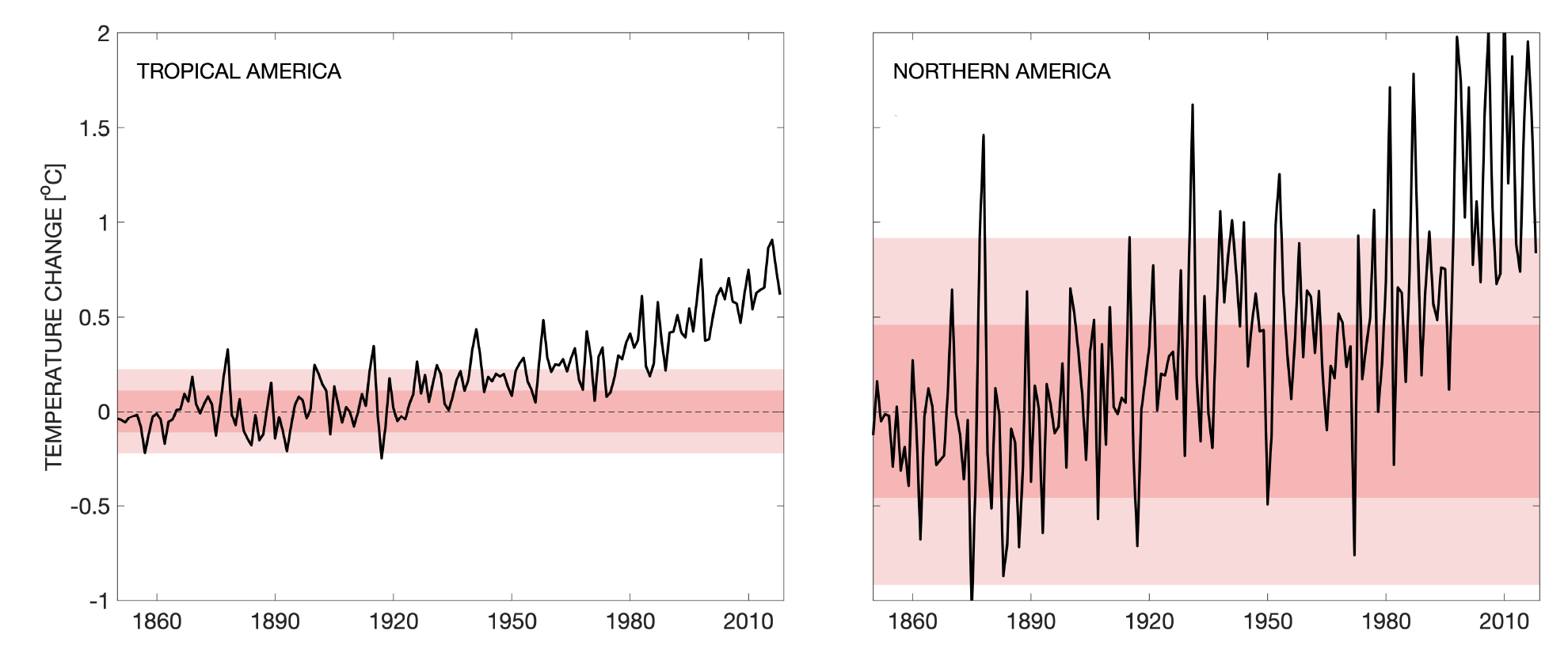
 Relative deviation. Though northern America has warmed more than its tropics, the tropics have more clearly departed from normal historical variability (colored bands: 1σ, 2σ standard deviations).[140]


_GISS.svg)


.gif)
In addition to global climate variability and global climate change over time, numerous climatic variations occur contemporaneously across different physical regions.
The oceans' absorption of about 90% of excess heat has helped to cause land surface temperatures to grow more rapidly than sea surface temperatures.[132] The Northern Hemisphere, having a larger landmass-to-ocean ratio than the Southern Hemisphere, shows greater average temperature increases.[134] Variations across different latitude bands also reflect this divergence in average temperature increase, with the temperature increase of northern extratropics exceeding that of the tropics, which in turn exceeds that of the southern extratropics.[135]
Upper regions of the atmosphere have been cooling contemporaneously with a warming in the lower atmosphere, confirming the action of the greenhouse effect and ozone depletion.[137]
Observed regional climatic variations confirm predictions concerning ongoing changes, for example, by contrasting (smoother) year-to-year global variations with (more volatile) year-to-year variations in localized regions.[138] Conversely, comparing different regions' warming patterns to their respective historical variabilities, allows the raw magnitudes of temperature changes to be placed in the perspective of what is normal variability for each region.[140]
Regional variability observations permit study of regionalized climate tipping points such as rainforest loss, ice sheet and sea ice melt, and permafrost thawing.[141] Such distinctions underlie research into a possible global cascade of tipping points.[141]
See also
[edit]Notes
[edit]- ^ America's Climate Choices: Panel on Advancing the Science of Climate Change; National Research Council (2010). Advancing the Science of Climate Change. Washington, D.C.: The National Academies Press. ISBN 978-0-309-14588-6. Archived from the original on 29 May 2014.
(p1) ... there is a strong, credible body of evidence, based on multiple lines of research, documenting that climate is changing and that these changes are in large part caused by human activities. While much remains to be learned, the core phenomenon, scientific questions, and hypotheses have been examined thoroughly and have stood firm in the face of serious scientific debate and careful evaluation of alternative explanations. (pp. 21–22) Some scientific conclusions or theories have been so thoroughly examined and tested, and supported by so many independent observations and results, that their likelihood of subsequently being found to be wrong is vanishingly small. Such conclusions and theories are then regarded as settled facts. This is the case for the conclusions that the Earth system is warming and that much of this warming is very likely due to human activities.
- ^ Rohli & Vega 2018, p. 274.
- ^ "The United Nations Framework Convention on Climate Change". 21 March 1994. Archived from the original on 20 September 2022. Retrieved 9 October 2018.
Climate change means a change of climate which is attributed directly or indirectly to human activity that alters the composition of the global atmosphere and which is in addition to natural climate variability observed over comparable time periods.
- ^ "What's in a Name? Global Warming vs. Climate Change". NASA. 5 December 2008. Archived from the original on 9 August 2010. Retrieved 23 July 2011.
- ^ a b Hulme, Mike (2016). "Concept of Climate Change, in: The International Encyclopedia of Geography". The International Encyclopedia of Geography. Wiley-Blackwell/Association of American Geographers (AAG): 1. Archived from the original on 29 September 2022. Retrieved 16 May 2016.
- ^ Hsiung, Jane (November 1985). "Estimates of Global Oceanic Meridional Heat Transport". Journal of Physical Oceanography. 15 (11): 1405–13. Bibcode:1985JPO....15.1405H. doi:10.1175/1520-0485(1985)015<1405:EOGOMH>2.0.CO;2.
- ^ Vallis, Geoffrey K.; Farneti, Riccardo (October 2009). "Meridional energy transport in the coupled atmosphere–ocean system: scaling and numerical experiments". Quarterly Journal of the Royal Meteorological Society. 135 (644): 1643–60. Bibcode:2009QJRMS.135.1643V. doi:10.1002/qj.498. S2CID 122384001.
- ^ Trenberth, Kevin E.; et al. (2009). "Earth's Global Energy Budget". Bulletin of the American Meteorological Society. 90 (3): 311–23. Bibcode:2009BAMS...90..311T. doi:10.1175/2008BAMS2634.1.
- ^ Smith, Ralph C. (2013). Uncertainty Quantification: Theory, Implementation, and Applications. Computational Science and Engineering. Vol. 12. SIAM. p. 23. ISBN 978-1-61197-322-8.
- ^ Cronin 2010, pp. 17–18
- ^ "Mean Monthly Temperature Records Across the Globe / Timeseries of Global Land and Ocean Areas at Record Levels for October from 1951–2023". NCEI.NOAA.gov. National Centers for Environmental Information (NCEI) of the National Oceanic and Atmospheric Administration (NOAA). November 2023. Archived from the original on 16 November 2023. (change "202310" in URL to see years other than 2023, and months other than 10=October)
- ^ Ruddiman 2008, pp. 261–62.
- ^ Hasselmann, K. (1976). "Stochastic climate models Part I. Theory". Tellus. 28 (6): 473–85. Bibcode:1976Tell...28..473H. doi:10.1111/j.2153-3490.1976.tb00696.x. ISSN 2153-3490.
- ^ Liu, Zhengyu (14 October 2011). "Dynamics of Interdecadal Climate Variability: A Historical Perspective". Journal of Climate. 25 (6): 1963–95. doi:10.1175/2011JCLI3980.1. ISSN 0894-8755. S2CID 53953041.
- ^ a b Ruddiman 2008, p. 262.
- ^ Benzi R, Parisi G, Sutera A, Vulpiani A (1982). "Stochastic resonance in climatic change". Tellus. 34 (1): 10–6. Bibcode:1982Tell...34...10B. doi:10.1111/j.2153-3490.1982.tb01787.x. Archived from the original on 1 December 2024.
- ^ Brown, Patrick T.; Li, Wenhong; Cordero, Eugene C.; Mauget, Steven A. (21 April 2015). "Comparing the model-simulated global warming signal to observations using empirical estimates of unforced noise". Scientific Reports. 5 (1): 9957. Bibcode:2015NatSR...5.9957B. doi:10.1038/srep09957. ISSN 2045-2322. PMC 4404682. PMID 25898351.
- ^ Hasselmann, K. (1 December 1976). "Stochastic climate models Part I. Theory". Tellus. 28 (6): 473–85. Bibcode:1976Tell...28..473H. doi:10.1111/j.2153-3490.1976.tb00696.x. ISSN 2153-3490.
- ^ Meehl, Gerald A.; Hu, Aixue; Arblaster, Julie M.; Fasullo, John; Trenberth, Kevin E. (8 April 2013). "Externally Forced and Internally Generated Decadal Climate Variability Associated with the Interdecadal Pacific Oscillation". Journal of Climate. 26 (18): 7298–310. Bibcode:2013JCli...26.7298M. doi:10.1175/JCLI-D-12-00548.1. ISSN 0894-8755. OSTI 1565088. S2CID 16183172. Archived from the original on 11 March 2023. Retrieved 5 June 2020.
- ^ England, Matthew H.; McGregor, Shayne; Spence, Paul; Meehl, Gerald A.; Timmermann, Axel; Cai, Wenju; Gupta, Alex Sen; McPhaden, Michael J.; Purich, Ariaan (1 March 2014). "Recent intensification of wind-driven circulation in the Pacific and the ongoing warming hiatus". Nature Climate Change. 4 (3): 222–27. Bibcode:2014NatCC...4..222E. doi:10.1038/nclimate2106. hdl:1959.4/unsworks_13554. ISSN 1758-678X.
- ^ Brown, Patrick T.; Li, Wenhong; Li, Laifang; Ming, Yi (28 July 2014). "Top-of-atmosphere radiative contribution to unforced decadal global temperature variability in climate models". Geophysical Research Letters. 41 (14) 2014GL060625. Bibcode:2014GeoRL..41.5175B. doi:10.1002/2014GL060625. hdl:10161/9167. ISSN 1944-8007. S2CID 16933795.
- ^ Palmer, M. D.; McNeall, D. J. (1 January 2014). "Internal variability of Earth's energy budget simulated by CMIP5 climate models". Environmental Research Letters. 9 (3) 034016. Bibcode:2014ERL.....9c4016P. doi:10.1088/1748-9326/9/3/034016. ISSN 1748-9326.
- ^ "El Niño & Other Oscillations". Woods Hole Oceanographic Institution. Archived from the original on 6 April 2019. Retrieved 6 April 2019.
- ^ Wang, Chunzai (2018). "A review of ENSO theories". National Science Review. 5 (6): 813–825. doi:10.1093/nsr/nwy104. ISSN 2095-5138.
- ^ Climate Prediction Center (19 December 2005). "ENSO FAQ: How often do El Niño and La Niña typically occur?". National Centers for Environmental Prediction. Archived from the original on 27 August 2009. Retrieved 26 July 2009.
- ^ Kevin Krajick. "Part of the Pacific Ocean Is Not Warming as Expected. Why". Columbia University Lamont-Doherty Earth Observatory. Archived from the original on 5 March 2023. Retrieved 2 November 2022.
- ^ Aristos Georgiou (26 June 2019). "Mystery Stretch of the Pacific Ocean Is Not Warming Like the Rest of the World's Waters". Newsweek. Archived from the original on 25 February 2023. Retrieved 2 November 2022.
- ^ "What is the MJO, and why do we care?". NOAA Climate.gov. Archived from the original on 15 March 2023. Retrieved 6 April 2019.
- ^ National Center for Atmospheric Research. Climate Analysis Section. Archived 22 June 2006 at the Wayback Machine Retrieved on 7 June 2007.
- ^ Baldwin, M. P.; Gray, L. J.; Dunkerton, T. J.; Hamilton, K.; Haynes, P. H.; Randel, W. J.; Holton, J. R.; Alexander, M. J.; Hirota, I. (2001). "The quasi-biennial oscillation". Reviews of Geophysics. 39 (2): 179–229. Bibcode:2001RvGeo..39..179B. doi:10.1029/1999RG000073. S2CID 16727059.
- ^ Newman, Matthew; Alexander, Michael A.; Ault, Toby R.; Cobb, Kim M.; Deser, Clara; Di Lorenzo, Emanuele; Mantua, Nathan J.; Miller, Arthur J.; Minobe, Shoshiro (2016). "The Pacific Decadal Oscillation, Revisited". Journal of Climate. 29 (12): 4399–4427. Bibcode:2016JCli...29.4399N. doi:10.1175/JCLI-D-15-0508.1. ISSN 0894-8755. S2CID 4824093.
- ^ "Interdecadal Pacific Oscillation". NIWA. 19 January 2016. Archived from the original on 17 March 2023. Retrieved 6 April 2019.
- ^ Kuijpers, Antoon; Bo Holm Jacobsen; Seidenkrantz, Marit-Solveig; Knudsen, Mads Faurschou (2011). "Tracking the Atlantic Multidecadal Oscillation through the last 8,000 years". Nature Communications. 2 (1): 178–. Bibcode:2011NatCo...2..178K. doi:10.1038/ncomms1186. ISSN 2041-1723. PMC 3105344. PMID 21285956.
- ^ Skonieczny, C. (2 January 2019). "Monsoon-driven Saharan dust variability over the past 240,000 years". Science Advances. 5 (1) eaav1887. Bibcode:2019SciA....5.1887S. doi:10.1126/sciadv.aav1887. PMC 6314818. PMID 30613782.
- ^ Thompson, David. "Annular Modes – Introduction". Archived from the original on 18 March 2023. Retrieved 11 February 2020.
- ^ Burroughs 2001, pp. 207–08.
- ^ Spracklen, D. V.; Bonn, B.; Carslaw, K. S. (2008). "Boreal forests, aerosols and the impacts on clouds and climate". Philosophical Transactions of the Royal Society A: Mathematical, Physical and Engineering Sciences. 366 (1885): 4613–26. Bibcode:2008RSPTA.366.4613S. doi:10.1098/rsta.2008.0201. PMID 18826917. S2CID 206156442.
- ^ Christner, B. C.; Morris, C. E.; Foreman, C. M.; Cai, R.; Sands, D. C. (2008). "Ubiquity of Biological Ice Nucleators in Snowfall" (PDF). Science. 319 (5867): 1214. Bibcode:2008Sci...319.1214C. doi:10.1126/science.1149757. PMID 18309078. S2CID 39398426. Archived (PDF) from the original on 5 March 2020.
- ^ Schwartzman, David W.; Volk, Tyler (1989). "Biotic enhancement of weathering and the habitability of Earth". Nature. 340 (6233): 457–60. Bibcode:1989Natur.340..457S. doi:10.1038/340457a0. S2CID 4314648.
- ^ Kopp, R.E.; Kirschvink, J.L.; Hilburn, I.A.; Nash, C.Z. (2005). "The Paleoproterozoic snowball Earth: A climate disaster triggered by the evolution of oxygenic photosynthesis". Proceedings of the National Academy of Sciences. 102 (32): 11131–36. Bibcode:2005PNAS..10211131K. doi:10.1073/pnas.0504878102. PMC 1183582. PMID 16061801.
- ^ Kasting, J.F.; Siefert, JL (2002). "Life and the Evolution of Earth's Atmosphere". Science. 296 (5570): 1066–68. Bibcode:2002Sci...296.1066K. doi:10.1126/science.1071184. PMID 12004117. S2CID 37190778.
- ^ Mora, C.I.; Driese, S.G.; Colarusso, L. A. (1996). "Middle to Late Paleozoic Atmospheric CO2 Levels from Soil Carbonate and Organic Matter". Science. 271 (5252): 1105–07. Bibcode:1996Sci...271.1105M. doi:10.1126/science.271.5252.1105. S2CID 128479221.
- ^ Berner, R.A. (1999). "Atmospheric oxygen over Phanerozoic time". Proceedings of the National Academy of Sciences. 96 (20): 10955–57. Bibcode:1999PNAS...9610955B. doi:10.1073/pnas.96.20.10955. PMC 34224. PMID 10500106.
- ^ Bains, Santo; Norris, Richard D.; Corfield, Richard M.; Faul, Kristina L. (2000). "Termination of global warmth at the Palaeocene/Eocene boundary through productivity feedback". Nature. 407 (6801): 171–74. Bibcode:2000Natur.407..171B. doi:10.1038/35025035. PMID 11001051. S2CID 4419536.
- ^ Zachos, J.C.; Dickens, G.R. (2000). "An assessment of the biogeochemical feedback response to the climatic and chemical perturbations of the LPTM". GFF. 122 (1): 188–89. Bibcode:2000GFF...122..188Z. doi:10.1080/11035890001221188. S2CID 129797785.
- ^ Speelman, E.N.; Van Kempen, M.M.L.; Barke, J.; Brinkhuis, H.; Reichart, G.J.; Smolders, A.J.P.; Roelofs, J.G.M.; Sangiorgi, F.; De Leeuw, J.W.; Lotter, A.F.; Sinninghe Damsté, J.S. (2009). "The Eocene Arctic Azolla bloom: Environmental conditions, productivity and carbon drawdown". Geobiology. 7 (2): 155–70. Bibcode:2009Gbio....7..155S. doi:10.1111/j.1472-4669.2009.00195.x. PMID 19323694. S2CID 13206343.
- ^ Brinkhuis, Henk; Schouten, Stefan; Collinson, Margaret E.; Sluijs, Appy; Sinninghe Damsté, Jaap S. Sinninghe; Dickens, Gerald R.; Huber, Matthew; Cronin, Thomas M.; Onodera, Jonaotaro; Takahashi, Kozo; Bujak, Jonathan P.; Stein, Ruediger; Van Der Burgh, Johan; Eldrett, James S.; Harding, Ian C.; Lotter, André F.; Sangiorgi, Francesca; Van Konijnenburg-Van Cittert, Han van Konijnenburg-van; De Leeuw, Jan W.; Matthiessen, Jens; Backman, Jan; Moran, Kathryn; Expedition 302, Scientists (2006). "Episodic fresh surface waters in the Eocene Arctic Ocean". Nature. 441 (7093): 606–09. Bibcode:2006Natur.441..606B. doi:10.1038/nature04692. hdl:11250/174278. PMID 16752440. S2CID 4412107.
{{cite journal}}: CS1 maint: numeric names: authors list (link) - ^ Retallack, Gregory J. (2001). "Cenozoic Expansion of Grasslands and Climatic Cooling". The Journal of Geology. 109 (4): 407–26. Bibcode:2001JG....109..407R. doi:10.1086/320791. S2CID 15560105.
- ^ Dutton, Jan F.; Barron, Eric J. (1997). "Miocene to present vegetation changes: A possible piece of the Cenozoic cooling puzzle". Geology. 25 (1): 39. Bibcode:1997Geo....25...39D. doi:10.1130/0091-7613(1997)025<0039:MTPVCA>2.3.CO;2.
- ^ Cronin 2010, p. 17
- ^ "3. Are human activities causing climate change?". science.org.au. Australian Academy of Science. Archived from the original on 8 May 2019. Retrieved 12 August 2017.
- ^ Antoaneta Yotova, ed. (2009). "Anthropogenic Climate Influences". Climate Change, Human Systems and Policy Volume I. Eolss Publishers. ISBN 978-1-905839-02-5. Archived from the original on 4 April 2023. Retrieved 16 August 2020.
- ^ Steinfeld, H.; P. Gerber; T. Wassenaar; V. Castel; M. Rosales; C. de Haan (2006). Livestock's long shadow. Archived from the original on 26 July 2008. Retrieved 21 July 2009.
- ^ The Editorial Board (28 November 2015). "What the Paris Climate Meeting Must Do". The New York Times. Archived from the original on 29 November 2015. Retrieved 28 November 2015.
- ^ "Volcanic Gases and Their Effects". U.S. Department of the Interior. 10 January 2006. Archived from the original on 1 August 2013. Retrieved 21 January 2008.
- ^ "Human Activities Emit Way More Carbon Dioxide Than Do Volcanoes". American Geophysical Union. 14 June 2011. Archived from the original on 9 May 2013. Retrieved 20 June 2011.
- ^ a b "Milankovitch Cycles and Glaciation". University of Montana. Archived from the original on 16 July 2011. Retrieved 2 April 2009.
- ^ Gale, Andrew S. (1989). "A Milankovitch scale for Cenomanian time". Terra Nova. 1 (5): 420–25. Bibcode:1989TeNov...1..420G. doi:10.1111/j.1365-3121.1989.tb00403.x.
- ^ "Same forces as today caused climate changes 1.4 billion years ago". sdu.dk. University of Denmark. Archived from the original on 12 March 2015.
- ^ a b van Nes, Egbert H.; Scheffer, Marten; Brovkin, Victor; Lenton, Timothy M.; Ye, Hao; Deyle, Ethan; Sugihara, George (2015). "Causal feedbacks in climate change". Nature Climate Change. 5 (5): 445–48. Bibcode:2015NatCC...5..445V. doi:10.1038/nclimate2568. ISSN 1758-6798.
- ^ Box 6.2: What Caused the Low Atmospheric Carbon Dioxide Concentrations During Glacial Times? Archived 8 January 2023 at the Wayback Machine in IPCC AR4 WG1 2007 .
- ^ a b Rohli & Vega 2018, p. 296.
- ^ Willson, Richard C.; Hudson, Hugh S. (1991). "The Sun's luminosity over a complete solar cycle". Nature. 351 (6321): 42–44. Bibcode:1991Natur.351...42W. doi:10.1038/351042a0. S2CID 4273483.
- ^ Turner, T. Edward; Swindles, Graeme T.; Charman, Dan J.; Langdon, Peter G.; Morris, Paul J.; Booth, Robert K.; Parry, Lauren E.; Nichols, Jonathan E. (5 April 2016). "Solar cycles or random processes? Evaluating solar variability in Holocene climate records". Scientific Reports. 6 (1) 23961. doi:10.1038/srep23961. ISSN 2045-2322. PMC 4820721. PMID 27045989.
- ^ Ribas, Ignasi (February 2010). The Sun and stars as the primary energy input in planetary atmospheres. IAU Symposium 264 'Solar and Stellar Variability – Impact on Earth and Planets'. Proceedings of the International Astronomical Union. Vol. 264. pp. 3–18. arXiv:0911.4872. Bibcode:2010IAUS..264....3R. doi:10.1017/S1743921309992298.
- ^ a b Marty, B. (2006). "Water in the Early Earth". Reviews in Mineralogy and Geochemistry. 62 (1): 421–450. Bibcode:2006RvMG...62..421M. doi:10.2138/rmg.2006.62.18.
- ^ Watson, E.B.; Harrison, TM (2005). "Zircon Thermometer Reveals Minimum Melting Conditions on Earliest Earth". Science. 308 (5723): 841–44. Bibcode:2005Sci...308..841W. doi:10.1126/science.1110873. PMID 15879213. S2CID 11114317.
- ^ Hagemann, Steffen G.; Gebre-Mariam, Musie; Groves, David I. (1994). "Surface-water influx in shallow-level Archean lode-gold deposits in Western, Australia". Geology. 22 (12): 1067. Bibcode:1994Geo....22.1067H. doi:10.1130/0091-7613(1994)022<1067:SWIISL>2.3.CO;2.
- ^ Sagan, C.; G. Mullen (1972). "Earth and Mars: Evolution of Atmospheres and Surface Temperatures". Science. 177 (4043): 52–6. Bibcode:1972Sci...177...52S. doi:10.1126/science.177.4043.52. PMID 17756316. S2CID 12566286. Archived from the original on 9 August 2010. Retrieved 30 January 2009.
- ^ Sagan, C.; Chyba, C (1997). "The Early Faint Sun Paradox: Organic Shielding of Ultraviolet-Labile Greenhouse Gases". Science. 276 (5316): 1217–21. Bibcode:1997Sci...276.1217S. doi:10.1126/science.276.5316.1217. PMID 11536805.
- ^ Schröder, K.-P.; Connon Smith, Robert (2008), "Distant future of the Sun and Earth revisited", Monthly Notices of the Royal Astronomical Society, 386 (1): 155–63, arXiv:0801.4031, Bibcode:2008MNRAS.386..155S, doi:10.1111/j.1365-2966.2008.13022.x, S2CID 10073988
- ^ a b Miles, M.G.; Grainger, R.G.; Highwood, E.J. (2004). "The significance of volcanic eruption strength and frequency for climate". Quarterly Journal of the Royal Meteorological Society. 130 (602): 2361–76. Bibcode:2004QJRMS.130.2361M. doi:10.1256/qj.03.60. S2CID 53005926.
- ^ "Volcanic Gases and Climate Change Overview". usgs.gov. USGS. Archived from the original on 29 July 2014. Retrieved 31 July 2014.
- ^ Annexes Archived 6 July 2019 at the Wayback Machine, in IPCC AR4 SYR 2008, p. 58.
- ^ Diggles, Michael (28 February 2005). "The Cataclysmic 1991 Eruption of Mount Pinatubo, Philippines". U.S. Geological Survey Fact Sheet 113-97. United States Geological Survey. Archived from the original on 25 August 2013. Retrieved 8 October 2009.
- ^ Diggles, Michael. "The Cataclysmic 1991 Eruption of Mount Pinatubo, Philippines". usgs.gov. Archived from the original on 25 August 2013. Retrieved 31 July 2014.
- ^ Oppenheimer, Clive (2003). "Climatic, environmental and human consequences of the largest known historic eruption: Tambora volcano (Indonesia) 1815". Progress in Physical Geography. 27 (2): 230–59. Bibcode:2003PrPG...27..230O. doi:10.1191/0309133303pp379ra. S2CID 131663534.
- ^ Black, Benjamin A.; Gibson, Sally A. (2019). "Deep Carbon and the Life Cycle of Large Igneous Provinces". Elements. 15 (5): 319–324. Bibcode:2019Eleme..15..319B. doi:10.2138/gselements.15.5.319.
- ^ Wignall, P (2001). "Large igneous provinces and mass extinctions". Earth-Science Reviews. 53 (1): 1–33. Bibcode:2001ESRv...53....1W. doi:10.1016/S0012-8252(00)00037-4.
- ^ Graf, H.-F.; Feichter, J.; Langmann, B. (1997). "Volcanic sulphur emissions: Estimates of source strength and its contribution to the global sulphate distribution". Journal of Geophysical Research: Atmospheres. 102 (D9): 10727–38. Bibcode:1997JGR...10210727G. doi:10.1029/96JD03265. hdl:21.11116/0000-0003-2CBB-A.
- ^ Forest, C.E.; Wolfe, J.A.; Molnar, P.; Emanuel, K.A. (1999). "Paleoaltimetry incorporating atmospheric physics and botanical estimates of paleoclimate". Geological Society of America Bulletin. 111 (4): 497–511. Bibcode:1999GSAB..111..497F. doi:10.1130/0016-7606(1999)111<0497:PIAPAB>2.3.CO;2. hdl:1721.1/10809.
- ^ "Panama: Isthmus that Changed the World". NASA Earth Observatory. Archived from the original on 2 August 2007. Retrieved 1 July 2008.
- ^ Haug, Gerald H.; Keigwin, Lloyd D. (22 March 2004). "How the Isthmus of Panama Put Ice in the Arctic". Oceanus. 42 (2). Woods Hole Oceanographic Institution. Archived from the original on 5 October 2018. Retrieved 1 October 2013.
- ^ Bruckschen, Peter; Oesmanna, Susanne; Veizer, Ján (30 September 1999). "Isotope stratigraphy of the European Carboniferous: proxy signals for ocean chemistry, climate and tectonics". Chemical Geology. 161 (1–3): 127–63. Bibcode:1999ChGeo.161..127B. doi:10.1016/S0009-2541(99)00084-4.
- ^ Parrish, Judith T. (1993). "Climate of the Supercontinent Pangea". The Journal of Geology. 101 (2). The University of Chicago Press: 215–33. Bibcode:1993JG....101..215P. doi:10.1086/648217. JSTOR 30081148. S2CID 128757269.
- ^ Hausfather, Zeke (18 August 2017). "Explainer: Why the sun is not responsible for recent climate change". Carbon Brief. Archived from the original on 17 March 2023. Retrieved 5 September 2019.
- ^ Pierce, J. R. (2017). "Cosmic rays, aerosols, clouds, and climate: Recent findings from the CLOUD experiment". Journal of Geophysical Research: Atmospheres. 122 (15): 8051–55. Bibcode:2017JGRD..122.8051P. doi:10.1002/2017JD027475. ISSN 2169-8996. S2CID 125580175.
- ^ Brugger, Julia; Feulner, Georg; Petri, Stefan (April 2017), "Severe environmental effects of Chicxulub impact imply key role in end-Cretaceous mass extinction", 19th EGU General Assembly, EGU2017, proceedings from the conference, 23–28 April 2017, vol. 19, Vienna, Austria, p. 17167, Bibcode:2017EGUGA..1917167B.
{{citation}}: CS1 maint: location missing publisher (link) - ^ Burroughs 2001, p. 232.
- ^ Hadlington, Simon 9 (May 2013). "Mineral dust plays key role in cloud formation and chemistry". Chemistry World. Archived from the original on 24 October 2022. Retrieved 5 September 2019.
{{cite web}}: CS1 maint: numeric names: authors list (link) - ^ Mahowald, Natalie; Albani, Samuel; Kok, Jasper F.; Engelstaeder, Sebastian; Scanza, Rachel; Ward, Daniel S.; Flanner, Mark G. (1 December 2014). "The size distribution of desert dust aerosols and its impact on the Earth system". Aeolian Research. 15: 53–71. Bibcode:2014AeoRe..15...53M. doi:10.1016/j.aeolia.2013.09.002. ISSN 1875-9637.
- ^ New, M.; Todd, M.; Hulme, M; Jones, P. (December 2001). "Review: Precipitation measurements and trends in the twentieth century". International Journal of Climatology. 21 (15): 1889–922. Bibcode:2001IJCli..21.1889N. doi:10.1002/joc.680. S2CID 56212756.
- ^ a b Demenocal, P.B. (2001). "Cultural Responses to Climate Change During the Late Holocene" (PDF). Science. 292 (5517): 667–73. Bibcode:2001Sci...292..667D. doi:10.1126/science.1059827. PMID 11303088. S2CID 18642937. Archived from the original (PDF) on 17 December 2008. Retrieved 28 August 2015.
- ^ Sindbaek, S.M. (2007). "Networks and nodal points: the emergence of towns in early Viking Age Scandinavia". Antiquity. 81 (311): 119–32. doi:10.1017/s0003598x00094886.
- ^ Dominic, F.; Burns, S.J.; Neff, U.; Mudulsee, M.; Mangina, A; Matter, A. (April 2004). "Palaeoclimatic interpretation of high-resolution oxygen isotope profiles derived from annually laminated speleothems from Southern Oman". Quaternary Science Reviews. 23 (7–8): 935–45. Bibcode:2004QSRv...23..935F. doi:10.1016/j.quascirev.2003.06.019.
- ^ Hughes, Malcolm K.; Swetnam, Thomas W.; Diaz, Henry F., eds. (2010). Dendroclimatology: progress and prospect. Developments in Paleoenvironmental Research. Vol. 11. New York: Springer Science & Business Media. ISBN 978-1-4020-4010-8.
- ^ Langdon, P.G.; Barber, K.E.; Lomas-Clarke, S.H.; Lomas-Clarke, S.H. (August 2004). "Reconstructing climate and environmental change in northern England through chironomid and pollen analyses: evidence from Talkin Tarn, Cumbria". Journal of Paleolimnology. 32 (2): 197–213. Bibcode:2004JPall..32..197L. doi:10.1023/B:JOPL.0000029433.85764.a5. S2CID 128561705.
- ^ Birks, H.H. (March 2003). "The importance of plant macrofossils in the reconstruction of Lateglacial vegetation and climate: examples from Scotland, western Norway, and Minnesota, US" (PDF). Quaternary Science Reviews. 22 (5–7): 453–73. Bibcode:2003QSRv...22..453B. doi:10.1016/S0277-3791(02)00248-2. hdl:1956/387. Archived from the original (PDF) on 11 June 2007. Retrieved 20 April 2018.
- ^ Miyoshi, N; Fujiki, Toshiyuki; Morita, Yoshimune (1999). "Palynology of a 250-m core from Lake Biwa: a 430,000-year record of glacial–interglacial vegetation change in Japan". Review of Palaeobotany and Palynology. 104 (3–4): 267–83. Bibcode:1999RPaPa.104..267M. doi:10.1016/S0034-6667(98)00058-X.
- ^ Prentice, I. Colin; Bartlein, Patrick J; Webb, Thompson (1991). "Vegetation and Climate Change in Eastern North America Since the Last Glacial Maximum". Ecology. 72 (6): 2038–56. Bibcode:1991Ecol...72.2038P. doi:10.2307/1941558. JSTOR 1941558.
- ^ Coope, G.R.; Lemdahl, G.; Lowe, J.J.; Walkling, A. (4 May 1999). "Temperature gradients in northern Europe during the last glacial – Holocene transition (14–9 14 C kyr BP) interpreted from coleopteran assemblages". Journal of Quaternary Science. 13 (5): 419–33. Bibcode:1998JQS....13..419C. doi:10.1002/(SICI)1099-1417(1998090)13:5<419::AID-JQS410>3.0.CO;2-D.
- ^ a b c Adams, J.M.; Faure, H., eds. (1997). "Global land environments since the last interglacial". Tennessee: Oak Ridge National Laboratory. Archived from the original on 16 January 2008. QEN members.
- ^ Swann, Abigail L. S. (1 June 2018). "Plants and Drought in a Changing Climate". Current Climate Change Reports. 4 (2): 192–201. Bibcode:2018CCCR....4..192S. doi:10.1007/s40641-018-0097-y. ISSN 2198-6061.
- ^ Ainsworth, E. A.; Lemonnier, P.; Wedow, J. M. (January 2020). Tausz-Posch, S. (ed.). "The influence of rising tropospheric carbon dioxide and ozone on plant productivity". Plant Biology. 22 (S1): 5–11. Bibcode:2020PlBio..22S...5A. doi:10.1111/plb.12973. ISSN 1435-8603. PMC 6916594. PMID 30734441.
- ^ Ochoa-Hueso, R; Delgado-Baquerizo, N; King, PTA; Benham, M; Arca, V; Power, SA (2019). "Ecosystem type and resource quality are more important than global change drivers in regulating early stages of litter decomposition". Soil Biology and Biochemistry. 129: 144–52. Bibcode:2019SBiBi.129..144O. doi:10.1016/j.soilbio.2018.11.009. hdl:10261/336676. S2CID 92606851.
- ^ Kinver, Mark (15 November 2011). "UK trees' fruit ripening '18 days earlier'". Bbc.co.uk. Archived from the original on 17 March 2023. Retrieved 1 November 2012.
- ^ a b Sahney, S.; Benton, M.J.; Falcon-Lang, H.J. (2010). "Rainforest collapse triggered Pennsylvanian tetrapod diversification in Euramerica" (PDF). Geology. 38 (12): 1079–82. Bibcode:2010Geo....38.1079S. doi:10.1130/G31182.1. Archived from the original on 17 March 2023. Retrieved 27 November 2013.
- ^ Bachelet, D.; Neilson, R.; Lenihan, J. M.; Drapek, R.J. (2001). "Climate Change Effects on Vegetation Distribution and Carbon Budget in the United States". Ecosystems. 4 (3): 164–85. Bibcode:2001Ecosy...4..164B. doi:10.1007/s10021-001-0002-7. S2CID 15526358.
- ^ Ridolfi, Luca; D'Odorico, P.; Porporato, A.; Rodriguez-Iturbe, I. (27 July 2000). "Impact of climate variability on the vegetation water stress". Journal of Geophysical Research: Atmospheres. 105 (D14): 18013–18025. Bibcode:2000JGR...10518013R. doi:10.1029/2000JD900206. ISSN 0148-0227.
- ^ Burroughs 2007, p. 273.
- ^ Millington, Rebecca; Cox, Peter M.; Moore, Jonathan R.; Yvon-Durocher, Gabriel (10 May 2019). "Modelling ecosystem adaptation and dangerous rates of global warming". Emerging Topics in Life Sciences. 3 (2): 221–31. doi:10.1042/ETLS20180113. hdl:10871/36988. ISSN 2397-8554. PMID 33523155. S2CID 150221323.
- ^ Burroughs 2007, p. 267.
- ^ Seiz, G.; N. Foppa (2007). The activities of the World Glacier Monitoring Service (WGMS) (PDF) (Report). Archived from the original (PDF) on 25 March 2009. Retrieved 21 June 2009.
- ^ "International Stratigraphic Chart". International Commission on Stratigraphy. 2008. Archived from the original on 15 October 2011. Retrieved 3 October 2011.
- ^ Burroughs 2007, p. 279.
- ^ Hansen, James. "Science Briefs: Earth's Climate History". NASA GISS. Archived from the original on 24 July 2011. Retrieved 25 April 2013.
- ^ Belt, Simon T.; Cabedo-Sanz, Patricia; Smik, Lukas; et al. (2015). "Identification of paleo Arctic winter sea ice limits and the marginal ice zone: Optimised biomarker-based reconstructions of late Quaternary Arctic sea ice". Earth and Planetary Science Letters. 431: 127–39. Bibcode:2015E&PSL.431..127B. doi:10.1016/j.epsl.2015.09.020. hdl:10026.1/4335. ISSN 0012-821X.
- ^ Warren, Stephen G.; Voigt, Aiko; Tziperman, Eli; et al. (1 November 2017). "Snowball Earth climate dynamics and Cryogenian geology-geobiology". Science Advances. 3 (11) e1600983. Bibcode:2017SciA....3E0983H. doi:10.1126/sciadv.1600983. ISSN 2375-2548. PMC 5677351. PMID 29134193.
- ^ Caballero, R.; Huber, M. (2013). "State-dependent climate sensitivity in past warm climates and its implications for future climate projections". Proceedings of the National Academy of Sciences. 110 (35): 14162–67. Bibcode:2013PNAS..11014162C. doi:10.1073/pnas.1303365110. ISSN 0027-8424. PMC 3761583. PMID 23918397.
- ^ Hansen James; Sato Makiko; Russell Gary; Kharecha Pushker (2013). "Climate sensitivity, sea level and atmospheric carbon dioxide". Philosophical Transactions of the Royal Society A: Mathematical, Physical and Engineering Sciences. 371 (2001) 20120294. arXiv:1211.4846. Bibcode:2013RSPTA.37120294H. doi:10.1098/rsta.2012.0294. PMC 3785813. PMID 24043864.
- ^ a b McInherney, F.A..; Wing, S. (2011). "A perturbation of carbon cycle, climate, and biosphere with implications for the future". Annual Review of Earth and Planetary Sciences. 39 (1): 489–516. Bibcode:2011AREPS..39..489M. doi:10.1146/annurev-earth-040610-133431. Archived from the original on 14 September 2016. Retrieved 26 October 2019.
- ^ Westerhold, T..; Röhl, U.; Raffi, I.; Fornaciari, E.; Monechi, S.; Reale, V.; Bowles, J.; Evans, H. F. (2008). "Astronomical calibration of the Paleocene time" (PDF). Palaeogeography, Palaeoclimatology, Palaeoecology. 257 (4): 377–403. Bibcode:2008PPP...257..377W. doi:10.1016/j.palaeo.2007.09.016. Archived (PDF) from the original on 9 August 2017.
- ^ Burroughs 2007, pp. 190–91.
- ^ Ivany, Linda C.; Pietsch, Carlie; Handley, John C.; Lockwood, Rowan; Allmon, Warren D.; Sessa, Jocelyn A. (1 September 2018). "Little lasting impact of the Paleocene-Eocene Thermal Maximum on shallow marine molluscan faunas". Science Advances. 4 (9) eaat5528. Bibcode:2018SciA....4.5528I. doi:10.1126/sciadv.aat5528. ISSN 2375-2548. PMC 6124918. PMID 30191179.
- ^ Haerter, Jan O.; Moseley, Christopher; Berg, Peter (2013). "Strong increase in convective precipitation in response to higher temperatures". Nature Geoscience. 6 (3): 181–85. Bibcode:2013NatGe...6..181B. doi:10.1038/ngeo1731. ISSN 1752-0908.
- ^ Kaufman, Darrell; McKay, Nicholas; Routson, Cody; Erb, Michael; Dätwyler, Christoph; Sommer, Philipp S.; Heiri, Oliver; Davis, Basil (30 June 2020). "Holocene global mean surface temperature, a multi-method reconstruction approach". Scientific Data. 7 (1): 201. Bibcode:2020NatSD...7..201K. doi:10.1038/s41597-020-0530-7. ISSN 2052-4463. PMC 7327079. PMID 32606396.
- ^ Zemp, M.; I.Roer; A.Kääb; M.Hoelzle; F.Paul; W. Haeberli (2008). United Nations Environment Programme – Global Glacier Changes: facts and figures (PDF) (Report). Archived from the original (PDF) on 25 March 2009. Retrieved 21 June 2009.
- ^ EPA, OA, US (July 2016). "Climate Change Indicators: Glaciers". US EPA. Archived from the original on 29 September 2019. Retrieved 26 January 2018.
- ^ "Land ice – NASA Global Climate Change". Archived from the original on 23 February 2017. Retrieved 10 December 2017.
- ^ Shaftel, Holly (ed.). "Climate Change: How do we know?". NASA Global Climate Change. Earth Science Communications Team at NASA's Jet Propulsion Laboratory. Archived from the original on 18 December 2019. Retrieved 16 December 2017.
- ^ "GISS Surface Temperature Analysis (v4) / Annual Mean Temperature Change over Land and over Ocean". NASA GISS. Archived from the original on 16 April 2020.
- ^ a b Harvey, Chelsea (1 November 2018). "The Oceans Are Heating Up Faster Than Expected". Scientific American. Archived from the original on 3 March 2020. Data from NASA GISS.
- ^ "GISS Surface Temperature Analysis (v4) / Annual Mean Temperature Change for Hemispheres". NASA GISS. Archived from the original on 16 April 2020.
- ^ a b Freedman, Andrew (9 April 2013). "In Warming, Northern Hemisphere is Outpacing the South". Climate Central. Archived from the original on 31 October 2019.
- ^ a b "GISS Surface Temperature Analysis (v4) / Temperature Change for Three Latitude Bands". NASA GISS. Archived from the original on 16 April 2020.
- ^ Hawkins, Ed; Williams, Richard G.; Young, Paul J.; Berardelli, Jeff; Burgess, Samantha N.; Highwood, Ellie; Randel, William; Roussenov, Vassil; Smith, Doug; Placky, Bernadette Woods (1 May 2025). "Warming Stripes Spark Climate Conversations: From the Ocean to the Stratosphere". Bulletin of the American Meteorological Society. 6 (5): E964 – E970. doi:10.1175/BAMS-D-24-0212.1.
- ^ a b Hawkins, Ed (12 September 2019). "Atmospheric temperature trends". Climate Lab Book. Archived from the original on 12 September 2019. (Higher-altitude cooling differences attributed to ozone depletion and greenhouse gas increases; spikes occurred with volcanic eruptions of 1982–83 (El Chichón) and 1991–92 (Pinatubo).)
- ^ a b Meduna, Veronika (17 September 2018). "The climate visualisations that leave no room for doubt or denial". The Spinoff. New Zealand. Archived from the original on 17 May 2019.
- ^ "Climate at a Glance / Global Time Series". NCDC / NOAA. Archived from the original on 23 February 2020.
- ^ a b Hawkins, Ed (10 March 2020). "From the familiar to the unknown". Climate Lab Book (professional blog). Archived from the original on 23 April 2020. (Direct link to image; Hawkins credits Berkeley Earth for data.) "The emergence of observed temperature changes over both land and ocean is clearest in tropical regions, in contrast to the regions of largest change which are in the northern extra-tropics. As an illustration, northern America has warmed more than tropical America, but the changes in the tropics are more apparent and have more clearly emerged from the range of historical variability. The year-to-year variations in the higher latitudes have made it harder to distinguish the long-term changes."
- ^ a b Lenton, Timothy M.; Rockström, Johan; Gaffney, Owen; Rahmstorf, Stefan; Richardson, Katherine; Steffen, Will; Schellnhuber, Hans Joachim (27 November 2019). "Climate tipping points – too risky to bet against". Nature. 575 (7784): 592–595. Bibcode:2019Natur.575..592L. doi:10.1038/d41586-019-03595-0. hdl:10871/40141. PMID 31776487. Correction dated 9 April 2020
References
[edit]- Cronin, Thomas N. (2010). Paleoclimates: understanding climate change past and present. New York: Columbia University Press. ISBN 978-0-231-14494-0.
- IPCC (2007). Solomon, S.; Qin, D.; Manning, M.; Chen, Z.; et al. (eds.). Climate Change 2007: The Physical Science Basis (PDF). Contribution of Working Group I to the Fourth Assessment Report of the Intergovernmental Panel on Climate Change. Cambridge University Press. ISBN 978-0-521-88009-1. (pb: ISBN 978-0-521-70596-7).
- IPCC (2008). The Core Writing Team; Pachauri, R.K.; Reisinger, A.R. (eds.). Climate Change 2008: Synthesis Report (PDF). Contribution of Working Groups I, II and III to the Fourth Assessment Report of the Intergovernmental Panel on Climate Change. Geneva, Switzerland: IPCC. ISBN 978-92-9169-122-7.
- Burroughs, William James (2001). Climate Change: A multidisciplinary approach. Cambridge: Cambridge university press. ISBN 0-521-56771-8.
- Burroughs, William James (2007). Climate Change: A multidisciplinary approach. Cambridge: Cambridge University Press. ISBN 978-0-511-37027-4.
- Ruddiman, William F. (2008). Earth's climate: Past and Future. New York: W. H. Freeman and Company. ISBN 978-0-7167-8490-6.
- Rohli, Robert. V.; Vega, Anthony J. (2018). Climatology (4th ed.). Jones & Bartlett Learning. ISBN 978-1-284-12656-3.
External links
[edit] Media related to Climate variability and change at Wikimedia Commons
- Global Climate Change from NASA (US)
- Intergovernmental Panel on Climate Change (IPCC)
- Climate Variability Archived 30 May 2023 at the Wayback Machine – NASA Science
- Climate Change and Variability, National Centers for Environmental Information Archived 21 September 2021 at the Wayback Machine
| Technological | |||||
|---|---|---|---|---|---|
| Sociological | |||||
| Ecological |
| ||||
| Biological |
| ||||
| Astronomical | |||||
| Eschatological | |||||
| Others |
| ||||
| Fictional | |||||
| Organizations | |||||
| General | |||||
Climate variability and change
View on GrokipediaTerminology and Concepts
Definitions of Variability and Change
Climate variability encompasses fluctuations in climate statistics, such as averages, extremes, and probabilities of temperature, precipitation, and other elements, occurring over timescales from seasons to several decades, distinct from individual weather events.[2] These variations arise primarily from internal atmospheric and oceanic processes, including phenomena like the El Niño-Southern Oscillation (ENSO), which redistribute heat and moisture globally, leading to temporary deviations from long-term norms without implying a permanent alteration in the climate's baseline state.[3] For instance, ENSO events can cause widespread drought or flooding on interannual scales, but they typically revert toward the mean over time.[2] In contrast, climate change denotes a long-term, statistically detectable shift in the mean state of the climate or its variability, persisting for periods of decades or longer, identifiable through methods like trend analysis or statistical tests.[14] This definition, as articulated by the Intergovernmental Panel on Climate Change (IPCC), encompasses changes attributable to both natural external forcings—such as solar irradiance variations or volcanic eruptions—and anthropogenic factors, including alterations to atmospheric composition from human emissions.[14] Unlike variability, which oscillates around a stable reference mean, climate change involves directional trends, such as sustained increases in global mean surface temperature observed since the late 19th century, exceeding natural variability thresholds in multiple datasets.[2][15] The demarcation between variability and change hinges on duration, persistence, and statistical significance: short-term anomalies (e.g., multi-year ENSO cycles) represent variability if they do not alter the underlying climate distribution, whereas prolonged shifts, like the Holocene warming or recent anthropogenic warming, qualify as change when they exceed historical ranges or demonstrate non-reverting trends.[2] This distinction is crucial for attribution studies, as natural variability can modulate or mask underlying change signals, requiring separation via modeling and paleoclimate proxies to discern causal drivers.[14] Sources emphasizing only human-induced aspects of change, such as certain policy-oriented reports, may understate natural precedents, but empirical records confirm climate has undergone multiple natural shifts over millennia, independent of human influence.[16]Key Metrics and Indicators
Global surface temperature anomalies serve as a primary indicator of climate variability and change, with datasets from NASA and NOAA showing the 2024 annual average at approximately 1.28°C above the 20th-century baseline, marking it as the warmest year on record.[17] This warming is modulated by natural oscillations like El Niño-Southern Oscillation (ENSO), which contributed to elevated temperatures in 2023-2024, though the long-term trend since 1880 reflects a rise of about 1.1°C.[6] For 2025 through August, global temperatures ranked second highest, trailing only 2024, amid a transition to neutral ENSO conditions.[18] Atmospheric carbon dioxide (CO₂) concentrations, measured at Mauna Loa Observatory, reached a monthly average of 425.48 ppm in August 2025, continuing an upward trajectory from 315 ppm in 1958, with annual increases accelerating due to anthropogenic emissions.[19] The May 2025 peak hit 430.2 ppm, the second-largest year-over-year jump in the 67-year record, underscoring persistent radiative forcing despite natural sinks absorbing roughly half of emissions.[20] Global mean sea level has risen at an average rate of 3.4 mm per year since 1993, as tracked by satellite altimetry, totaling 8-9 inches (21-24 cm) since 1880, driven by thermal expansion and land ice melt.[21] In 2024, the rate accelerated beyond expectations, linked to extreme ocean warming, reaching a record high of 101.4 mm above 1993 levels by year-end.[22] [23] Upper ocean heat content has increased steadily since the 1970s, absorbing over 90% of Earth's excess energy, with the top 2000 meters gaining heat at rates exceeding prior decades, as evidenced by Argo float and ship-based measurements.[24] This accumulation, equivalent to roughly four Hiroshima bombs per second in recent years, reflects both radiative imbalance and ocean circulation changes.[25] Arctic sea ice minimum extent reached 4.60 million square kilometers in September 2025, tying for the 10th lowest in the satellite era (since 1979), with a long-term decline of 12.2% per decade amid reduced summer melt onset and extent.[26] Variability from weather patterns and ENSO influences annual minima, but the trend indicates diminished ice volume and thickness.[27] Other indicators include shifts in precipitation extremes and drought indices, such as the U.S. Climate Extremes Index, which tracks departures in temperature, precipitation, and drought, showing increased frequency of extremes in recent decades, though regional patterns vary due to internal variability.[28] These metrics, derived from instrumental records and proxies, quantify changes against natural baselines but require accounting for data adjustments and urban heat effects in surface observations.[29]Natural Drivers
Internal Climate Variability
Internal climate variability refers to natural fluctuations in the climate system arising from chaotic internal dynamics and interactions among components such as the atmosphere, oceans, land surface, and cryosphere, without requiring external forcings.[30] These processes generate preferred spatial patterns of variability, known as modes, that operate on timescales from intraseasonal to multidecadal and contribute substantially to climate predictability on subseasonal to decadal horizons.[30] Internal variability is generally larger in the extratropics than tropics and stronger in winter than summer, influencing regional weather patterns and masking forced trends in short-term observations.[31] The El Niño-Southern Oscillation (ENSO) represents a dominant interannual mode, with cycles typically lasting 2-7 years, driven by coupled ocean-atmosphere interactions in the tropical Pacific.[30] During El Niño phases, enhanced easterly trade winds weaken, leading to warmer sea surface temperatures (SSTs) in the central-eastern Pacific, which shift the Walker circulation and generate global teleconnections affecting precipitation and temperature; for instance, El Niño events have been linked to increased hurricane activity in the Pacific and droughts in Indonesia.[30] La Niña phases, conversely, feature cooler SSTs and strengthened trades, often resulting in opposite impacts, such as floods in Peru and drier conditions in the southern U.S.[30] ENSO variability accounts for much of the year-to-year global temperature fluctuations, with strong events capable of altering annual averages by up to 0.15°C.[30] Decadal to multidecadal modes include the Pacific Decadal Oscillation (PDO), characterized by SST anomalies in the North Pacific north of 20°N, with phases shifting roughly every 20-30 years.[32] Positive PDO phases feature cooling in the central North Pacific and warming along the coasts, impacting marine ecosystems, such as reduced salmon catches during cool phases, and modulating North American precipitation patterns.[32] The PDO enhances El Niño teleconnections to North America during positive phases, amplifying winter precipitation in the southwestern U.S. and diminishing La Niña effects.[33] The Atlantic Multidecadal Oscillation (AMO) exhibits SST variability in the North Atlantic on 60-80 year cycles, with warm phases since the mid-1990s linked to heightened Atlantic hurricane frequency and intensified multidecadal ENSO variability through alterations in the annual cycle.[34] AMO warm periods increase drought risk in the U.S. Southwest and north-central regions, while also influencing Sahel rainfall; for example, the positive AMO phase correlates with stronger Pacific ITCZ variability.[35] [36] These oscillations arise from internal ocean circulation changes, such as variations in the Atlantic Meridional Overturning Circulation, rather than direct radiative forcing.[34] Internal modes like ENSO, PDO, and AMO introduce substantial uncertainty in attributing regional climate changes, as their amplitudes can rival anthropogenic forcing on decadal scales, particularly over land areas where variability is amplified.[37] For instance, natural decadal variations may equal global warming-induced surface air temperature changes in magnitude for regional predictions.[37] While models simulate these modes, debates persist on their exact internal origins versus subtle external influences, with some analyses questioning robust multidecadal oscillations in unforced simulations.[38] Nonetheless, observational and modeling evidence confirms their role in generating low-frequency variability that overlays long-term trends.[39]
External Natural Forcings
External natural forcings encompass variations in solar output, volcanic aerosol emissions, and Earth's orbital parameters that alter the planetary energy balance independently of internal climate dynamics. These factors have driven significant climate shifts across geological timescales, with solar and volcanic influences affecting decadal to centennial variability, while orbital changes operate on millennial scales. Empirical reconstructions indicate their radiative forcings are typically small in the modern era compared to pre-industrial baselines but have modulated past climates through direct energetic imbalances.[40][41][42] Solar irradiance variations, tracked via sunspot cycles and proxy records, impose a radiative forcing of about ±0.17 W/m² over the 11-year Schwabe cycle, stemming from a 0.1% fluctuation in total solar irradiance. This equates to global temperature responses of roughly 0.1°C, as observed in satellite measurements since 1978 showing no net upward trend in irradiance amid rising temperatures. Longer-term solar minima, such as the Maunder Minimum (1645–1715), correlated with cooler European winters, but reconstructions attribute only modest global cooling of 0.1–0.3°C, underscoring limited efficacy for explaining centennial-scale changes without amplification mechanisms like cosmic ray-induced cloud cover, which remain debated.[43][44][45] Orbital forcings, formalized by Milankovitch, arise from eccentricity (100,000-year cycle modulating perihelion distance), obliquity (41,000-year axial tilt variation affecting seasonal contrast), and precession (23,000-year wobble shifting solstice timing). These redistribute insolation, with high-latitude summer peaks driving glacial terminations; for instance, obliquity maxima increase Northern Hemisphere insolation by up to 50 W/m² at 65°N, initiating deglaciations as seen in oxygen isotope records from ice cores. In the Holocene, declining obliquity has favored a gradual cooling trajectory, projecting multi-millennial declines of 0.5–1°C per 5,000 years absent countervailing influences, incompatible with 20th-century warming patterns.[46][47][48] Volcanic forcings occur via stratospheric sulfate aerosol veils from sulfur-rich eruptions, scattering incoming shortwave radiation and yielding negative forcings of 1–5 W/m² for 1–3 years. The 1991 Mount Pinatubo eruption exemplifies this, injecting 20 million tons of SO₂ and inducing 0.5°C global cooling detectable in surface temperatures. Larger historical events, like the 1815 Tambora blast, amplified aerosol lifetimes through self-lofting, but aggregate volcanic forcing over the 20th century nets near-zero due to episodic nature, contributing to short-term dips amid longer trends rather than sustained directional change.[49][50][51]Anthropogenic Factors
Greenhouse Gas Contributions
Anthropogenic greenhouse gas emissions arise predominantly from fossil fuel combustion, industrial processes, agriculture, waste management, and land-use changes such as deforestation. These activities have elevated atmospheric concentrations of long-lived greenhouse gases, with carbon dioxide (CO2), methane (CH4), and nitrous oxide (N2O) comprising the majority. Fluorinated gases, though minor in volume, possess high global warming potentials. Global anthropogenic GHG emissions reached 52.9 GtCO2e in 2023, reflecting a 62% increase since 1990.[52] CO2 accounts for approximately 74-76% of total anthropogenic GHG emissions in CO2-equivalent terms, primarily from fossil fuel oxidation in energy production, transportation, and industry, supplemented by cement manufacturing and net land-use emissions. Fossil fuel-related CO2 emissions totaled about 37 Gt in 2023, with coal, oil, and natural gas as key contributors; land-use changes, including deforestation, added roughly 4-5 GtCO2 annually in recent years, though net land sinks partially offset this.[53][54][55]| Greenhouse Gas | Approximate Share of Total Anthropogenic Emissions (CO2e, %) | Primary Anthropogenic Sources |
|---|---|---|
| CO2 | 74.5 (fossil) + land-use contributions | Fossil fuel combustion, cement production, deforestation[55][54] |
| CH4 | 17.9 | Enteric fermentation in livestock, rice cultivation, fossil fuel extraction and leaks, landfills[55][56] |
| N2O | 4 | Agricultural soil management (fertilizers), manure, industrial processes[55][52] |
| Fluorinated gases | ~2-3 | Industrial refrigerants, aerosols, semiconductors[57][58] |